Effect of variables' uncertainties on the uncertainty of a function based on them
統計学 において 、 不確実性の伝播とは、 変数 の 不確実性が、それらに基づく 関数 の不確実性に及ぼす 影響のことです 。変数が実験測定の値である場合、測定限界 (例えば、機器の 精度) に起因する不確実性が あり、関数内の変数の組み合わせによって伝播します。
不確実性 u は 、さまざまな方法で表現できます。 絶対誤差 Δ x で定義できます。不確実性は、 相対誤差 (Δ x )/ x で定義することもでき、通常はパーセントで表されます。最も一般的な方法は、量の不確実性は標準偏差 σ ( 分散 の正の平方根) で定量化されます 。量の値とその誤差は、区間 x ± u として表現されます。ただし、不確実性を特徴付ける最も一般的な方法は、 確率分布 を指定することです。変数の 確率分布 が既知であるか仮定できる場合は、理論的にはその統計量のいずれかを取得することができます。特に、 変数の真の値が存在する領域を説明する 信頼限界を導くことが可能です。たとえば、 正規分布 に属する 1 次元変数の 68% 信頼限界は、 中心値 x から約 ± 1 標準偏差 σ です。つまり、領域 x ± σ は、およそ 68% のケースで真の値をカバーすることになります。
不確実性に 相関が ある場合、 共分散を 考慮する必要があります。相関は2つの異なる原因から生じます。1つ目は、 測定誤差が 相関している場合です。2つ目は、基礎となる値が母集団全体で相関している場合、 グループ平均の不確実性 も相関するということです。 [1]
非線形関数が不確実なパラメータ(相関の有無にかかわらず)を変更する一般的な状況では、不確実性を伝播し、結果として生じる量の確率分布/統計を推測するための標準的なツールは、 モンテカルロ法 ファミリーのサンプリング手法です。 [2] 非常に大きなデータセットや複雑な関数の場合、誤差伝播の計算に非常にコストがかかる可能性があるため、 代替モデル [3] または 並列計算 戦略 [4] [5] [6] が必要になる場合があります。
特定のケースでは、不確実性の伝播計算は単純な代数的手法で行うことができます。以下に、こうしたシナリオのいくつかを説明します。
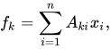
線形結合 をm 個の関数の集合とし 、これらは 結合係数を持つ 変数 の線形結合である 。 または行列表記では、 { f k ( x 1 , x 2 , … , x n ) } {\displaystyle \{f_{k}(x_{1},x_{2},\dots ,x_{n})\}} n {\displaystyle n} x 1 , x 2 , … , x n {\displaystyle x_{1},x_{2},\dots ,x_{n}} A k 1 , A k 2 , … , A k n , ( k = 1 , … , m ) {\displaystyle A_{k1},A_{k2},\dots ,A_{kn},(k=1,\dots ,m)} f k = ∑ i = 1 n A k i x i , {\displaystyle f_{k}=\sum _{i=1}^{n}A_{ki}x_{i},} f = A x . {\displaystyle \mathbf {f} =\mathbf {A} \mathbf {x} .}
また、 x = ( x 1 , ..., x n ) の 分散共分散行列 を で表し 、平均値を で表すとします 。
は 外積 です 。 Σ x {\displaystyle {\boldsymbol {\Sigma }}^{x}} μ {\displaystyle {\boldsymbol {\mu }}} Σ x = E [ ( x − μ ) ⊗ ( x − μ ) ] = ( σ 1 2 σ 12 σ 13 ⋯ σ 21 σ 2 2 σ 23 ⋯ σ 31 σ 32 σ 3 2 ⋯ ⋮ ⋮ ⋮ ⋱ ) = ( Σ 11 x Σ 12 x Σ 13 x ⋯ Σ 21 x Σ 22 x Σ 23 x ⋯ Σ 31 x Σ 32 x Σ 33 x ⋯ ⋮ ⋮ ⋮ ⋱ ) . {\displaystyle {\begin{aligned}{\boldsymbol {\Sigma }}^{x}=\operatorname {E} [(\mathbf {x} -{\boldsymbol {\mu }})\otimes (\mathbf {x} -{\boldsymbol {\mu }})]&={\begin{pmatrix}\sigma _{1}^{2}&\sigma _{12}&\sigma _{13}&\cdots \\\sigma _{21}&\sigma _{2}^{2}&\sigma _{23}&\cdots \\\sigma _{31}&\sigma _{32}&\sigma _{3}^{2}&\cdots \\\vdots &\vdots &\vdots &\ddots \end{pmatrix}}\\[1ex]&={\begin{pmatrix}{\Sigma }_{11}^{x}&{\Sigma }_{12}^{x}&{\Sigma }_{13}^{x}&\cdots \\{\Sigma }_{21}^{x}&{\Sigma }_{22}^{x}&{\Sigma }_{23}^{x}&\cdots \\{\Sigma }_{31}^{x}&{\Sigma }_{32}^{x}&{\Sigma }_{33}^{x}&\cdots \\\vdots &\vdots &\vdots &\ddots \end{pmatrix}}.\end{aligned}}} ⊗ {\displaystyle \otimes }
そして、 f の 分散共分散行列 は次のように与えられる。 Σ f {\displaystyle {\boldsymbol {\Sigma }}^{f}} Σ f = E [ ( f − E [ f ] ) ⊗ ( f − E [ f ] ) ] = E [ A ( x − μ ) ⊗ A ( x − μ ) ] = A E [ ( x − μ ) ⊗ ( x − μ ) ] A T = A Σ x A T . {\displaystyle {\begin{aligned}{\boldsymbol {\Sigma }}^{f}&=\operatorname {E} \left[(\mathbf {f} -\operatorname {E} [\mathbf {f} ])\otimes (\mathbf {f} -\operatorname {E} [\mathbf {f} ])\right]=\operatorname {E} \left[\mathbf {A} (\mathbf {x} -{\boldsymbol {\mu }})\otimes \mathbf {A} (\mathbf {x} -{\boldsymbol {\mu }})\right]\\[1ex]&=\mathbf {A} \operatorname {E} \left[(\mathbf {x} -{\boldsymbol {\mu }})\otimes (\mathbf {x} -{\boldsymbol {\mu }})\right]\mathbf {A} ^{\mathrm {T} }=\mathbf {A} {\boldsymbol {\Sigma }}^{x}\mathbf {A} ^{\mathrm {T} }.\end{aligned}}}
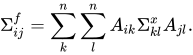
成分表記では、この式 は Σ f = A Σ x A T {\displaystyle {\boldsymbol {\Sigma }}^{f}=\mathbf {A} {\boldsymbol {\Sigma }}^{x}\mathbf {A} ^{\mathrm {T} }} Σ i j f = ∑ k n ∑ l n A i k Σ k l x A j l . {\displaystyle \Sigma _{ij}^{f}=\sum _{k}^{n}\sum _{l}^{n}A_{ik}{\Sigma }_{kl}^{x}A_{jl}.}
これは、ある変数群から別の変数群への誤差の伝播を表す最も一般的な表現です。 x の誤差が無相関の場合、この一般表現は次のように簡略化されます
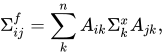
。 ここで、 は xベクトルの k 番目の要素 の分散です。 x の誤差が無相関であっても、 f の誤差は 一般に相関していることに注意してください。言い換えれば、が 対角行列 であっても 、 は一般に非線形行列です。 Σ i j f = ∑ k n A i k Σ k x A j k , {\displaystyle \Sigma _{ij}^{f}=\sum _{k}^{n}A_{ik}\Sigma _{k}^{x}A_{jk},} Σ k x = σ x k 2 {\displaystyle \Sigma _{k}^{x}=\sigma _{x_{k}}^{2}} Σ x {\displaystyle {\boldsymbol {\Sigma }}^{x}} Σ f {\displaystyle {\boldsymbol {\Sigma }}^{f}}
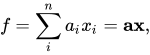
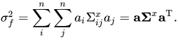
スカラー値関数 f の一般的な表現は少し単純です (ここで a は行ベクトルです)。 f = ∑ i n a i x i = a x , {\displaystyle f=\sum _{i}^{n}a_{i}x_{i}=\mathbf {ax} ,} σ f 2 = ∑ i n ∑ j n a i Σ i j x a j = a Σ x a T . {\displaystyle \sigma _{f}^{2}=\sum _{i}^{n}\sum _{j}^{n}a_{i}\Sigma _{ij}^{x}a_{j}=\mathbf {a} {\boldsymbol {\Sigma }}^{x}\mathbf {a} ^{\mathrm {T} }.}
各共分散項は 相関係数 を用いて 次のように表すことができる。したがって、 f の分散の別の表現は次のように なる。 σ i j {\displaystyle \sigma _{ij}} ρ i j {\displaystyle \rho _{ij}} σ i j = ρ i j σ i σ j {\displaystyle \sigma _{ij}=\rho _{ij}\sigma _{i}\sigma _{j}} σ f 2 = ∑ i n a i 2 σ i 2 + ∑ i n ∑ j ( j ≠ i ) n a i a j ρ i j σ i σ j . {\displaystyle \sigma _{f}^{2}=\sum _{i}^{n}a_{i}^{2}\sigma _{i}^{2}+\sum _{i}^{n}\sum _{j(j\neq i)}^{n}a_{i}a_{j}\rho _{ij}\sigma _{i}\sigma _{j}.}
x の変数が無相関の場合 、これはさらに次のように単純化される。 σ f 2 = ∑ i n a i 2 σ i 2 . {\displaystyle \sigma _{f}^{2}=\sum _{i}^{n}a_{i}^{2}\sigma _{i}^{2}.}
係数と分散が同一の単純なケースでは、 σ f = n | a | σ . {\displaystyle \sigma _{f}={\sqrt {n}}\,|a|\sigma .}
算術平均の場合 、結果は 平均の標準誤差 になります。 a = 1 / n {\displaystyle a=1/n} σ f = σ n . {\displaystyle \sigma _{f}={\frac {\sigma }{\sqrt {n}}}.}
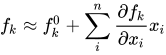
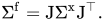
非線形結合 f が変数 x の非線形結合の集合である 場合 、 変数のすべての整合した値を含む区間を計算するために、 区間伝播を実行できます。確率的アプローチでは、関数 f は通常、1次 テイラー級数 展開の近似によって線形化する必要がありますが、場合によっては、積の正確な分散の場合のように、展開に依存しない正確な式を導出できます。 [7] テイラー展開は次のようになります。 ここで、 は、ベクトル xのすべての要素の平均値で評価された、 i 番目の変数 に関する f k の 偏微分を 表します 。または、 行列表記 では となり、 J は ヤコビ行列 です。 f 0 は定数であるため、 f の誤差には寄与しません。したがって、誤差の伝播は上記の線形の場合に従いますが、線形係数 A ki と A kj を偏微分と に置き換え ます 。行列表記では、 [8] f k ≈ f k 0 + ∑ i n ∂ f k ∂ x i x i {\displaystyle f_{k}\approx f_{k}^{0}+\sum _{i}^{n}{\frac {\partial f_{k}}{\partial {x_{i}}}}x_{i}} ∂ f k / ∂ x i {\displaystyle \partial f_{k}/\partial x_{i}} f ≈ f 0 + J x {\displaystyle \mathrm {f} \approx \mathrm {f} ^{0}+\mathrm {J} \mathrm {x} \,} ∂ f k ∂ x i {\displaystyle {\frac {\partial f_{k}}{\partial x_{i}}}} ∂ f k ∂ x j {\displaystyle {\frac {\partial f_{k}}{\partial x_{j}}}} Σ f = J Σ x J ⊤ . {\displaystyle \mathrm {\Sigma } ^{\mathrm {f} }=\mathrm {J} \mathrm {\Sigma } ^{\mathrm {x} }\mathrm {J} ^{\top }.}
つまり、関数のヤコビアンを用いて、引数の分散共分散行列の行と列を変換します。これは、 を用いた線形の場合の行列式と等価であることに注意してください 。 J = A {\displaystyle \mathrm {J=A} }
簡素化 相関関係を無視したり独立変数を仮定したりすると、誤差の伝播を計算するためのエンジニアや実験科学者の間で共通の式、分散式が得られます。 [9] ここで、は 関数の標準偏差を表し 、 はの標準偏差を表し 、 はの標準偏差を表し 、などとなります。 s f = ( ∂ f ∂ x ) 2 s x 2 + ( ∂ f ∂ y ) 2 s y 2 + ( ∂ f ∂ z ) 2 s z 2 + ⋯ {\displaystyle s_{f}={\sqrt {\left({\frac {\partial f}{\partial x}}\right)^{2}s_{x}^{2}+\left({\frac {\partial f}{\partial y}}\right)^{2}s_{y}^{2}+\left({\frac {\partial f}{\partial z}}\right)^{2}s_{z}^{2}+\cdots }}} s f {\displaystyle s_{f}} f {\displaystyle f} s x {\displaystyle s_{x}} x {\displaystyle x} s y {\displaystyle s_{y}} y {\displaystyle y}
この式は の勾配の線形特性に基づいており、 が十分に小さい 限り、 の標準偏差の良好な推定値となります。具体的には、 の 線形近似 は、半径 の近傍範囲内 で に近い値を取る必要があります 。 [10] f {\displaystyle f} f {\displaystyle f} s x , s y , s z , … {\displaystyle s_{x},s_{y},s_{z},\ldots } f {\displaystyle f} f {\displaystyle f} s x , s y , s z , … {\displaystyle s_{x},s_{y},s_{z},\ldots }
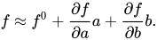
例 2変数の 非線形 微分可能関数 、 、 は 、 と展開できます。 両辺の分散を取り、 変数の線形結合の分散について
公式 [11] を使用すると、次の式
が得られます。 ここで 、 は関数 の標準偏差 、 は の標準偏差 、 は の標準偏差 、は と の共分散です 。 f ( a , b ) {\displaystyle f(a,b)} a {\displaystyle a} b {\displaystyle b} f ≈ f 0 + ∂ f ∂ a a + ∂ f ∂ b b . {\displaystyle f\approx f^{0}+{\frac {\partial f}{\partial a}}a+{\frac {\partial f}{\partial b}}b.} Var ( a X + b Y ) = a 2 Var ( X ) + b 2 Var ( Y ) + 2 a b Cov ( X , Y ) , {\displaystyle \operatorname {Var} (aX+bY)=a^{2}\operatorname {Var} (X)+b^{2}\operatorname {Var} (Y)+2ab\operatorname {Cov} (X,Y),} σ f 2 ≈ | ∂ f ∂ a | 2 σ a 2 + | ∂ f ∂ b | 2 σ b 2 + 2 ∂ f ∂ a ∂ f ∂ b σ a b , {\displaystyle \sigma _{f}^{2}\approx \left|{\frac {\partial f}{\partial a}}\right|^{2}\sigma _{a}^{2}+\left|{\frac {\partial f}{\partial b}}\right|^{2}\sigma _{b}^{2}+2{\frac {\partial f}{\partial a}}{\frac {\partial f}{\partial b}}\sigma _{ab},} σ f {\displaystyle \sigma _{f}} f {\displaystyle f} σ a {\displaystyle \sigma _{a}} a {\displaystyle a} σ b {\displaystyle \sigma _{b}} b {\displaystyle b} σ a b = σ a σ b ρ a b {\displaystyle \sigma _{ab}=\sigma _{a}\sigma _{b}\rho _{ab}} a {\displaystyle a} b {\displaystyle b}
、、 という特定のケースでは 、 と の間に相関関係がある か 、 または です 。 f = a b {\displaystyle f=ab} ∂ f ∂ a = b {\displaystyle {\frac {\partial f}{\partial a}}=b} ∂ f ∂ b = a {\displaystyle {\frac {\partial f}{\partial b}}=a} σ f 2 ≈ b 2 σ a 2 + a 2 σ b 2 + 2 a b σ a b {\displaystyle \sigma _{f}^{2}\approx b^{2}\sigma _{a}^{2}+a^{2}\sigma _{b}^{2}+2ab\,\sigma _{ab}} ( σ f f ) 2 ≈ ( σ a a ) 2 + ( σ b b ) 2 + 2 ( σ a a ) ( σ b b ) ρ a b {\displaystyle \left({\frac {\sigma _{f}}{f}}\right)^{2}\approx \left({\frac {\sigma _{a}}{a}}\right)^{2}+\left({\frac {\sigma _{b}}{b}}\right)^{2}+2\left({\frac {\sigma _{a}}{a}}\right)\left({\frac {\sigma _{b}}{b}}\right)\rho _{ab}} ρ a b {\displaystyle \rho _{ab}} a {\displaystyle a} b {\displaystyle b}
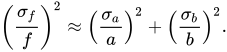
変数 とが 無相関の場合 、 a {\displaystyle a} b {\displaystyle b} ρ a b = 0 {\displaystyle \rho _{ab}=0} ( σ f f ) 2 ≈ ( σ a a ) 2 + ( σ b b ) 2 . {\displaystyle \left({\frac {\sigma _{f}}{f}}\right)^{2}\approx \left({\frac {\sigma _{a}}{a}}\right)^{2}+\left({\frac {\sigma _{b}}{b}}\right)^{2}.}
注意点と警告 非線形関数の誤差推定値は、 打ち切り級数展開を用いるため、 バイアスが生じます。このバイアスの程度は関数の性質に依存します。例えば、log(1+ x ) について計算された誤差のバイアスは、 x が 増加するにつれて大きくなります。これは、 x への展開が 良好な近似値となるのは、 x が ゼロに近い場合のみであるためです。
高度に非線形な関数の場合、不確実性の伝播に対する確率的アプローチには5つのカテゴリが存在します。 [12] 詳細については 不確実性の定量化を 参照してください。
逆数とシフト逆数 逆数または逆数の特殊なケース 、つまり 標準正規分布 に従う場合 、結果として得られる分布は逆数標準正規分布であり、定義可能な分散は存在しません。 [13] 1 / B {\displaystyle 1/B} B = N ( 0 , 1 ) {\displaystyle B=N(0,1)}
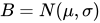
しかし、一般的な正規分布に従うシフト逆関数のやや一般的なケースでは、極と平均の差が実数値であれば、平均と分散の統計量は主値の意味で 存在 し ます 。 [ 14 ] 1 / ( p − B ) {\displaystyle 1/(p-B)} B = N ( μ , σ ) {\displaystyle B=N(\mu ,\sigma )} p {\displaystyle p} μ {\displaystyle \mu }
比率 比率にも問題があり、特定の条件下では正規近似値が存在します。
この表は、実変数の単純な関数の分散と標準偏差を 標準偏差 共分散 と相関とともに示している。 実数値係数 とが 正確に既知(決定論的)であると仮定されている。すなわち、 A , B {\displaystyle A,B} σ A , σ B , {\displaystyle \sigma _{A},\sigma _{B},} σ A B = ρ A B σ A σ B , {\displaystyle \sigma _{AB}=\rho _{AB}\sigma _{A}\sigma _{B},} ρ A B . {\displaystyle \rho _{AB}.} a {\displaystyle a} b {\displaystyle b} σ a = σ b = 0. {\displaystyle \sigma _{a}=\sigma _{b}=0.}
表の右側の列では、 と は 期待値 であり 、 は それらの値で計算された関数の値です。 A {\displaystyle A} B {\displaystyle B} f {\displaystyle f}
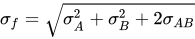
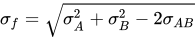
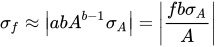
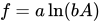
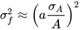
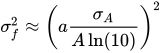
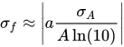
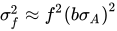
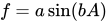
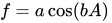
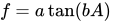
関数 分散 標準偏差 f = a A {\displaystyle f=aA\,} σ f 2 = a 2 σ A 2 {\displaystyle \sigma _{f}^{2}=a^{2}\sigma _{A}^{2}} σ f = | a | σ A {\displaystyle \sigma _{f}=|a|\sigma _{A}} f = A + B {\displaystyle f=A+B} σ f 2 = σ A 2 + σ B 2 + 2 σ A B {\displaystyle \sigma _{f}^{2}=\sigma _{A}^{2}+\sigma _{B}^{2}+2\sigma _{AB}} σ f = σ A 2 + σ B 2 + 2 σ A B {\displaystyle \sigma _{f}={\sqrt {\sigma _{A}^{2}+\sigma _{B}^{2}+2\sigma _{AB}}}} f = A − B {\displaystyle f=A-B} σ f 2 = σ A 2 + σ B 2 − 2 σ A B {\displaystyle \sigma _{f}^{2}=\sigma _{A}^{2}+\sigma _{B}^{2}-2\sigma _{AB}} σ f = σ A 2 + σ B 2 − 2 σ A B {\displaystyle \sigma _{f}={\sqrt {\sigma _{A}^{2}+\sigma _{B}^{2}-2\sigma _{AB}}}} f = a A + b B {\displaystyle f=aA+bB} σ f 2 = a 2 σ A 2 + b 2 σ B 2 + 2 a b σ A B {\displaystyle \sigma _{f}^{2}=a^{2}\sigma _{A}^{2}+b^{2}\sigma _{B}^{2}+2ab\,\sigma _{AB}} σ f = a 2 σ A 2 + b 2 σ B 2 + 2 a b σ A B {\displaystyle \sigma _{f}={\sqrt {a^{2}\sigma _{A}^{2}+b^{2}\sigma _{B}^{2}+2ab\,\sigma _{AB}}}} f = a A − b B {\displaystyle f=aA-bB} σ f 2 = a 2 σ A 2 + b 2 σ B 2 − 2 a b σ A B {\displaystyle \sigma _{f}^{2}=a^{2}\sigma _{A}^{2}+b^{2}\sigma _{B}^{2}-2ab\,\sigma _{AB}} σ f = a 2 σ A 2 + b 2 σ B 2 − 2 a b σ A B {\displaystyle \sigma _{f}={\sqrt {a^{2}\sigma _{A}^{2}+b^{2}\sigma _{B}^{2}-2ab\,\sigma _{AB}}}} f = A B {\displaystyle f=AB} σ f 2 ≈ f 2 [ ( σ A A ) 2 + ( σ B B ) 2 + 2 σ A B A B ] {\displaystyle \sigma _{f}^{2}\approx f^{2}\left[\left({\frac {\sigma _{A}}{A}}\right)^{2}+\left({\frac {\sigma _{B}}{B}}\right)^{2}+2{\frac {\sigma _{AB}}{AB}}\right]} [15] [16] σ f ≈ | f | ( σ A A ) 2 + ( σ B B ) 2 + 2 σ A B A B {\displaystyle \sigma _{f}\approx \left|f\right|{\sqrt {\left({\frac {\sigma _{A}}{A}}\right)^{2}+\left({\frac {\sigma _{B}}{B}}\right)^{2}+2{\frac {\sigma _{AB}}{AB}}}}} f = A B {\displaystyle f={\frac {A}{B}}} σ f 2 ≈ f 2 [ ( σ A A ) 2 + ( σ B B ) 2 − 2 σ A B A B ] {\displaystyle \sigma _{f}^{2}\approx f^{2}\left[\left({\frac {\sigma _{A}}{A}}\right)^{2}+\left({\frac {\sigma _{B}}{B}}\right)^{2}-2{\frac {\sigma _{AB}}{AB}}\right]} [17] σ f ≈ | f | ( σ A A ) 2 + ( σ B B ) 2 − 2 σ A B A B {\displaystyle \sigma _{f}\approx \left|f\right|{\sqrt {\left({\frac {\sigma _{A}}{A}}\right)^{2}+\left({\frac {\sigma _{B}}{B}}\right)^{2}-2{\frac {\sigma _{AB}}{AB}}}}} f = A A + B {\displaystyle f={\frac {A}{A+B}}} σ f 2 ≈ f 2 ( A + B ) 2 ( B 2 A 2 σ A 2 + σ B 2 − 2 B A σ A B ) {\displaystyle \sigma _{f}^{2}\approx {\frac {f^{2}}{\left(A+B\right)^{2}}}\left({\frac {B^{2}}{A^{2}}}\sigma _{A}^{2}+\sigma _{B}^{2}-2{\frac {B}{A}}\sigma _{AB}\right)} σ f ≈ | f A + B | B 2 A 2 σ A 2 + σ B 2 − 2 B A σ A B {\displaystyle \sigma _{f}\approx \left|{\frac {f}{A+B}}\right|{\sqrt {{\frac {B^{2}}{A^{2}}}\sigma _{A}^{2}+\sigma _{B}^{2}-2{\frac {B}{A}}\sigma _{AB}}}} f = a A b {\displaystyle f=aA^{b}} σ f 2 ≈ ( a b A b − 1 σ A ) 2 = ( f b σ A A ) 2 {\displaystyle \sigma _{f}^{2}\approx \left({a}{b}{A}^{b-1}{\sigma _{A}}\right)^{2}=\left({\frac {{f}{b}{\sigma _{A}}}{A}}\right)^{2}} σ f ≈ | a b A b − 1 σ A | = | f b σ A A | {\displaystyle \sigma _{f}\approx \left|{a}{b}{A}^{b-1}{\sigma _{A}}\right|=\left|{\frac {{f}{b}{\sigma _{A}}}{A}}\right|} f = a ln ( b A ) {\displaystyle f=a\ln(bA)} σ f 2 ≈ ( a σ A A ) 2 {\displaystyle \sigma _{f}^{2}\approx \left(a{\frac {\sigma _{A}}{A}}\right)^{2}} [18] σ f ≈ | a σ A A | {\displaystyle \sigma _{f}\approx \left|a{\frac {\sigma _{A}}{A}}\right|} f = a log 10 ( b A ) {\displaystyle f=a\log _{10}(bA)} σ f 2 ≈ ( a σ A A ln ( 10 ) ) 2 {\displaystyle \sigma _{f}^{2}\approx \left(a{\frac {\sigma _{A}}{A\ln(10)}}\right)^{2}} [18] σ f ≈ | a σ A A ln ( 10 ) | {\displaystyle \sigma _{f}\approx \left|a{\frac {\sigma _{A}}{A\ln(10)}}\right|} f = a e b A {\displaystyle f=ae^{bA}} σ f 2 ≈ f 2 ( b σ A ) 2 {\displaystyle \sigma _{f}^{2}\approx f^{2}\left(b\sigma _{A}\right)^{2}} [19] σ f ≈ | f | | ( b σ A ) | {\displaystyle \sigma _{f}\approx \left|f\right|\left|\left(b\sigma _{A}\right)\right|} f = a b A {\displaystyle f=a^{bA}} σ f 2 ≈ f 2 ( b ln ( a ) σ A ) 2 {\displaystyle \sigma _{f}^{2}\approx f^{2}(b\ln(a)\sigma _{A})^{2}} σ f ≈ | f | | b ln ( a ) σ A | {\displaystyle \sigma _{f}\approx \left|f\right|\left|b\ln(a)\sigma _{A}\right|} f = a sin ( b A ) {\displaystyle f=a\sin(bA)} σ f 2 ≈ [ a b cos ( b A ) σ A ] 2 {\displaystyle \sigma _{f}^{2}\approx \left[ab\cos(bA)\sigma _{A}\right]^{2}} σ f ≈ | a b cos ( b A ) σ A | {\displaystyle \sigma _{f}\approx \left|ab\cos(bA)\sigma _{A}\right|} f = a cos ( b A ) {\displaystyle f=a\cos \left(bA\right)\,} σ f 2 ≈ [ a b sin ( b A ) σ A ] 2 {\displaystyle \sigma _{f}^{2}\approx \left[ab\sin(bA)\sigma _{A}\right]^{2}} σ f ≈ | a b sin ( b A ) σ A | {\displaystyle \sigma _{f}\approx \left|ab\sin(bA)\sigma _{A}\right|} f = a tan ( b A ) {\displaystyle f=a\tan \left(bA\right)\,} σ f 2 ≈ [ a b sec 2 ( b A ) σ A ] 2 {\displaystyle \sigma _{f}^{2}\approx \left[ab\sec ^{2}(bA)\sigma _{A}\right]^{2}} σ f ≈ | a b sec 2 ( b A ) σ A | {\displaystyle \sigma _{f}\approx \left|ab\sec ^{2}(bA)\sigma _{A}\right|} f = A B {\displaystyle f=A^{B}} σ f 2 ≈ f 2 [ ( B A σ A ) 2 + ( ln ( A ) σ B ) 2 + 2 B ln ( A ) A σ A B ] {\displaystyle \sigma _{f}^{2}\approx f^{2}\left[\left({\frac {B}{A}}\sigma _{A}\right)^{2}+\left(\ln(A)\sigma _{B}\right)^{2}+2{\frac {B\ln(A)}{A}}\sigma _{AB}\right]} σ f ≈ | f | ( B A σ A ) 2 + ( ln ( A ) σ B ) 2 + 2 B ln ( A ) A σ A B {\displaystyle \sigma _{f}\approx \left|f\right|{\sqrt {\left({\frac {B}{A}}\sigma _{A}\right)^{2}+\left(\ln(A)\sigma _{B}\right)^{2}+2{\frac {B\ln(A)}{A}}\sigma _{AB}}}} f = a A 2 ± b B 2 {\displaystyle f={\sqrt {aA^{2}\pm bB^{2}}}} σ f 2 ≈ ( A f ) 2 a 2 σ A 2 + ( B f ) 2 b 2 σ B 2 ± 2 a b A B f 2 σ A B {\displaystyle \sigma _{f}^{2}\approx \left({\frac {A}{f}}\right)^{2}a^{2}\sigma _{A}^{2}+\left({\frac {B}{f}}\right)^{2}b^{2}\sigma _{B}^{2}\pm 2ab{\frac {AB}{f^{2}}}\,\sigma _{AB}} σ f ≈ ( A f ) 2 a 2 σ A 2 + ( B f ) 2 b 2 σ B 2 ± 2 a b A B f 2 σ A B {\displaystyle \sigma _{f}\approx {\sqrt {\left({\frac {A}{f}}\right)^{2}a^{2}\sigma _{A}^{2}+\left({\frac {B}{f}}\right)^{2}b^{2}\sigma _{B}^{2}\pm 2ab{\frac {AB}{f^{2}}}\,\sigma _{AB}}}}
相関のない変数( , )の場合、より複雑な関数の式は、より単純な関数を組み合わせることで導出できます。例えば、相関がないと仮定して繰り返し乗算を行うと、 ρ A B = 0 {\displaystyle \rho _{AB}=0} σ A B = 0 {\displaystyle \sigma _{AB}=0} f = A B C ; ( σ f f ) 2 ≈ ( σ A A ) 2 + ( σ B B ) 2 + ( σ C C ) 2 . {\displaystyle f=ABC;\qquad \left({\frac {\sigma _{f}}{f}}\right)^{2}\approx \left({\frac {\sigma _{A}}{A}}\right)^{2}+\left({\frac {\sigma _{B}}{B}}\right)^{2}+\left({\frac {\sigma _{C}}{C}}\right)^{2}.}
の場合、正確な分散についてはグッドマンの式 [7] も成り立ちます 。相関のない場合には、となり 、したがって、 最後の項は、両辺をで割ることでわかるように、通常の式に対する小さな修正を表しています 。 f = A B {\displaystyle f=AB} V [ X Y ] = E [ X ] 2 V [ Y ] + E [ Y ] 2 V [ X ] + V [ X ] V [ Y ] , {\displaystyle \operatorname {V} [XY]=\operatorname {E} [X]^{2}\operatorname {V} [Y]+\operatorname {E} [Y]^{2}\operatorname {V} [X]+\operatorname {V} [X]\operatorname {V} [Y],} σ f 2 = A 2 σ B 2 + B 2 σ A 2 + σ A 2 σ B 2 . {\displaystyle \sigma _{f}^{2}=A^{2}\sigma _{B}^{2}+B^{2}\sigma _{A}^{2}+\sigma _{A}^{2}\sigma _{B}^{2}.} f 2 = A 2 B 2 {\displaystyle f^{2}=A^{2}B^{2}} ( σ f f ) 2 = ( σ A A ) 2 + ( σ B B ) 2 + ( σ A σ B A B ) 2 . {\displaystyle \left({\frac {\sigma _{f}}{f}}\right)^{2}=\left({\frac {\sigma _{A}}{A}}\right)^{2}+\left({\frac {\sigma _{B}}{B}}\right)^{2}+\left({\frac {\sigma _{A}\sigma _{B}}{AB}}\right)^{2}.}
相関関係が差異に与える影響 A と B が無相関の場合 、両者の差 A − B の分散は、どちらよりも大きくなります。正の相関( )が増加すると、差の分散は減少し、完全に相関した変数が 同じ分散 を持つ場合、分散はゼロに収束します。一方、負の相関( )は、無相関の場合と比較して、差の分散をさらに増加させます。 ρ A B → 1 {\displaystyle \rho _{AB}\to 1} ρ A B → − 1 {\displaystyle \rho _{AB}\to -1}
例えば、自己減算 f = A − A は、変量が完全に 自己相関して いる場合( )にのみ 分散がゼロになります。A が 無相関の場合、 出力分散は入力分散の2倍になります。 また、 A が完全に反相関の場合、 出力では入力分散の4倍になります ( 上記の表の f = aA − aA に注目してください)。 σ f 2 = 0 {\displaystyle \sigma _{f}^{2}=0} ρ A = 1 {\displaystyle \rho _{A}=1} ρ A = 0 , {\displaystyle \rho _{A}=0,} σ f 2 = 2 σ A 2 . {\displaystyle \sigma _{f}^{2}=2\sigma _{A}^{2}.} ρ A = − 1 , {\displaystyle \rho _{A}=-1,} σ f 2 = 4 σ A 2 {\displaystyle \sigma _{f}^{2}=4\sigma _{A}^{2}} 1 − ρ A = 2 {\displaystyle 1-\rho _{A}=2}
計算例
逆正接関数 偏微分を使用して誤差を伝播する例として、逆正接関数の不確実性の伝播を計算できます。
x の測定における絶対不確かさを どこ に 定義する
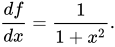
か。f ( x )の x に関する 微分 は f ( x ) = arctan ( x ) , {\displaystyle f(x)=\arctan(x),} Δ x {\displaystyle \Delta _{x}} d f d x = 1 1 + x 2 . {\displaystyle {\frac {df}{dx}}={\frac {1}{1+x^{2}}}.}
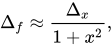
したがって、伝播された不確実性は、 絶対的な伝播された不確実性がある 場所です。 Δ f ≈ Δ x 1 + x 2 , {\displaystyle \Delta _{f}\approx {\frac {\Delta _{x}}{1+x^{2}}},} Δ f {\displaystyle \Delta _{f}}
抵抗測定 実際の応用としては、 オームの法則 R = V / I を 使用して 抵抗 R を 決定するために 、 抵抗器の 電流 I と 電圧 V を 測定 する 実験 があります。
不確実性を伴う測定変数 I ± σ I と V ± σ V が与えられ、それらの相関関係を無視すると、計算量 σ R の不確実性は次のようになります。
σ R ≈ σ V 2 ( 1 I ) 2 + σ I 2 ( − V I 2 ) 2 = R ( σ V V ) 2 + ( σ I I ) 2 . {\displaystyle \sigma _{R}\approx {\sqrt {\sigma _{V}^{2}\left({\frac {1}{I}}\right)^{2}+\sigma _{I}^{2}\left({\frac {-V}{I^{2}}}\right)^{2}}}=R{\sqrt {\left({\frac {\sigma _{V}}{V}}\right)^{2}+\left({\frac {\sigma _{I}}{I}}\right)^{2}}}.}
参照
参考文献 ^ キルヒナー、ジェームズ. 「データ分析ツールキット #5:不確実性分析と誤差伝播」 (PDF) . バークレー地震学研究所 . カリフォルニア大学. 2016年 4月22日 閲覧 。 ^ Kroese, DP; Taimre, T.; Botev, ZI (2011). モンテカルロ法ハンドブック . John Wiley & Sons. ^ ランフトル, サシャ; フォン・デア・リンデン, ヴォルフガング (2021年11月13日). 「ベイズ代理分析と不確実性の伝播」. 物理科学フォーラム . 3 (1): 6. arXiv : 2101.04038 . doi : 10.3390/psf2021003006 . ISSN 2673-9984. ^ Atanassova, E.; Gurov, T.; Karaivanova, A.; Ivanovska, S.; Durchova, M.; Dimitrov, D. (2016). 「Intel MICアーキテクチャにおける並列化アプローチについて」 AIP Conference Proceedings . 1773 (1): 070001. Bibcode :2016AIPC.1773g0001A. doi :10.1063/1.4964983. ^ Cunha Jr, A.; Nasser, R.; Sampaio, R.; Lopes, H.; Breitman, K. (2014). 「クラウドコンピューティング環境におけるモンテカルロ法による不確実性の定量化」. Computer Physics Communications . 185 (5): 1355– 1363. arXiv : 2105.09512 . Bibcode :2014CoPhC.185.1355C. doi :10.1016/j.cpc.2014.01.006. S2CID 32376269. ^ Lin, Y.; Wang, F.; Liu, B. (2018). 「FPGA上での大規模並列モンテカルロシミュレーションのための乱数ジェネレーター」. Journal of Computational Physics . 360 : 93–103 . Bibcode :2018JCoPh.360...93L. doi :10.1016/j.jcp.2018.01.029. ^ ab グッドマン、レオ (1960). 「製品の正確な分散について」. アメリカ統計学会誌 . 55 (292): 708– 713. doi :10.2307/2281592. JSTOR 2281592. ^ Ochoa1, Benjamin; Belongie, Serge「ガイド付きマッチングのための共分散伝播」2011年7月20日アーカイブ、 Wayback Machine ^ Ku, HH (1966年10月). 「誤差伝播式の使用に関する注記」. 米国国立標準技術研究所ジャーナル . 70C (4): 262. doi : 10.6028/jres.070c.025 . ISSN 0022-4316 . 2012年 10月3日 閲覧 。 ^ Clifford, AA (1973). 多変量誤差解析:多パラメータシステムにおける誤差伝播と計算のハンドブック . John Wiley & Sons. ISBN 978-0470160558 。 [ ページが必要 ] ^ Soch, Joram (2020年7月7日). 「2つの確率変数の線形結合の分散」. 『統計的証明の書』 . 2022年1月29日 閲覧 。 ^ Lee, SH; Chen, W. (2009). 「ブラックボックス型問題における不確実性伝播手法の比較研究」. 構造最適化と多分野最適化 . 37 (3): 239– 253. doi :10.1007/s00158-008-0234-7. S2CID 119988015. ^ ジョンソン、ノーマン・L.、コッツ、サミュエル、バラクリシュナン、ナラヤナスワミ (1994). 連続一変量分布、第1巻 . Wiley. p. 171. ISBN 0-471-58495-9 。 ^ ルコント, クリストフ (2013年5月). 「不確実性を伴うシステムの正確な統計:ランク1確率動的システムの解析理論」. Journal of Sound and Vibration . 332 (11): 2750– 2776. Bibcode :2013JSV...332.2750L. doi :10.1016/j.jsv.2012.12.009. ^ 「エラー伝播の概要」 (PDF) p. 2。 2016年12月13日時点の オリジナル (PDF)からアーカイブ。 2016年4月4日 閲覧 。 ^ 「数学的演算による不確実性の伝播」 (PDF) 5ページ。 2016年4月4日 閲覧 。 ^ 「分散推定のための戦略」 (PDF) 37ページ。 2013年1月18日 閲覧 。 ^ ab Harris, Daniel C. (2003), 定量化学分析(第6版)、Macmillan、p. 56、 ISBN 978-0-7167-4464-1 ^ 「エラー伝播チュートリアル」 (PDF) . フットヒルカレッジ . 2009年10月9日. 2012年3月1日 閲覧 。
さらに読む ベヴィントン、フィリップ・R.; ロビンソン、D.キース (2002)、 『物理科学のためのデータ整理と誤差分析』 (第3版)、マグロウヒル、 ISBN 978-0-07-119926-1 フォルナシーニ、パオロ(2008)、物理的測定における不確実性:物理学実験室におけるデータ分析入門、シュプリンガー、p. 161、 ISBN 978-0-387-78649-0 マイヤー、スチュアート L. (1975)、 『科学者とエンジニアのためのデータ分析』 、Wiley、 ISBN 978-0-471-59995-1 Peralta, M. (2012) 「 誤差の伝播:測定誤差を数学的に予測する方法 」CreateSpace Rouaud, M. (2013)、「確率、統計、推定:実験測定における不確実性の伝播」 (PDF) (短縮版) テイラー、JR(1997年)、 誤差解析入門:物理的測定における不確かさの研究 (第2版)、University Science Books Wang, CM; Iyer, Hari K. (2005-09-07). 「伝播する不確実性に対する高次補正について」. Metrologia . 42 (5): 406– 410. Bibcode :2005Metro..42..406W. doi :10.1088/0026-1394/42/5/011. ISSN 0026-1394. S2CID 122841691.
外部リンク 測定と不確実性の伝播に関する詳細な議論。単純な有意性演算の代わりに誤差伝播式とモンテカルロシミュレーションを使用する利点を説明する。 GUM、測定における不確かさの表現に関するガイド EPFL 誤差伝播、導出、意味、および Cy = Fx Cx Fx' の例の紹介 不確実性パッケージは、不確実性(および誤差相関)を含む計算を透過的に実行するためのプログラム/ライブラリです。 soerp パッケージは、不確実性 (およびエラー相関) を伴う *2 次* 計算を透過的に実行するための Python プログラム/ライブラリです。 計量ガイド合同委員会 (2011). JCGM 102: 測定データの評価 - 「測定における不確かさの表現に関するガイド」補足2 - 任意の数の出力量への拡張 (PDF) (技術レポート). JCGM . 2013年 2月13日 閲覧 . 不確実性計算機 任意の表現の不確実性を伝播する






![{\displaystyle {\begin{aligned}{\boldsymbol {\Sigma }}^{x}=\operatorname {E} [(\mathbf {x} -{\boldsymbol {\mu }})\otimes (\mathbf {x} -{\boldsymbol {\mu }})]&={\begin{pmatrix}\sigma _{1}^{2}&\sigma _{12}&\sigma _{13}&\cdots \\\sigma _{21}&\sigma _{2}^{2}&\sigma _{23}&\cdots \\\sigma _{31}&\sigma _{32}&\sigma _{3}^{2}&\cdots \\\vdots &\vdots &\vdots &\ddots \end{pmatrix}}\\[1ex]&={\begin{pmatrix}{\Sigma }_{11}^{x}&{\Sigma }_{12}^{x}&{\Sigma }_{13}^{x}&\cdots \\{\Sigma }_{21}^{x}&{\Sigma }_{22}^{x}&{\Sigma }_{23}^{x}&\cdots \\{\Sigma }_{31}^{x}&{\Sigma }_{32}^{x}&{\Sigma }_{33}^{x}&\cdots \\\vdots &\vdots &\vdots &\ddots \end{pmatrix}}.\end{aligned}}}](https://wikimedia.org/api/rest_v1/media/math/render/svg/ef96443b3a74cb0d40e8488eed779239a706232d)


![{\displaystyle {\begin{aligned}{\boldsymbol {\Sigma }}^{f}&=\operatorname {E} \left[(\mathbf {f} -\operatorname {E} [\mathbf {f} ])\otimes (\mathbf {f} -\operatorname {E} [\mathbf {f} ])\right]=\operatorname {E} \left[\mathbf {A} (\mathbf {x} -{\boldsymbol {\mu }})\otimes \mathbf {A} (\mathbf {x} -{\boldsymbol {\mu }})\right]\\[1ex]&=\mathbf {A} \operatorname {E} \left[(\mathbf {x} -{\boldsymbol {\mu }})\otimes (\mathbf {x} -{\boldsymbol {\mu }})\right]\mathbf {A} ^{\mathrm {T} }=\mathbf {A} {\boldsymbol {\Sigma }}^{x}\mathbf {A} ^{\mathrm {T} }.\end{aligned}}}](https://wikimedia.org/api/rest_v1/media/math/render/svg/6707679f9d88c2e9ff12f76463e050801b32812d)












































![{\displaystyle \sigma _{f}^{2}\approx f^{2}\left[\left({\frac {\sigma _{A}}{A}}\right)^{2}+\left({\frac {\sigma _{B}}{B}}\right)^{2}+2{\frac {\sigma _{AB}}{AB}}\right]}](https://wikimedia.org/api/rest_v1/media/math/render/svg/9499339791864087918a8411cfc3d6d3d64adb4d)


![{\displaystyle \sigma _{f}^{2}\approx f^{2}\left[\left({\frac {\sigma _{A}}{A}}\right)^{2}+\left({\frac {\sigma _{B}}{B}}\right)^{2}-2{\frac {\sigma _{AB}}{AB}}\right]}](https://wikimedia.org/api/rest_v1/media/math/render/svg/1443509fb7b51ea477c6c24a17910bde4e81863a)













![{\displaystyle \sigma _{f}^{2}\approx \left[ab\cos(bA)\sigma _{A}\right]^{2}}](https://wikimedia.org/api/rest_v1/media/math/render/svg/02967f1c0ff2eb7edac9b2fad3bb020fb7fad0cf)

![{\displaystyle \sigma _{f}^{2}\approx \left[ab\sin(bA)\sigma _{A}\right]^{2}}](https://wikimedia.org/api/rest_v1/media/math/render/svg/4f4d187dd08f03fd8b03cf3606cc9f166e5656aa)

![{\displaystyle \sigma _{f}^{2}\approx \left[ab\sec ^{2}(bA)\sigma _{A}\right]^{2}}](https://wikimedia.org/api/rest_v1/media/math/render/svg/4308e87b0ada5699f04d64d6088e12e18fc7511f)


![{\displaystyle \sigma _{f}^{2}\approx f^{2}\left[\left({\frac {B}{A}}\sigma _{A}\right)^{2}+\left(\ln(A)\sigma _{B}\right)^{2}+2{\frac {B\ln(A)}{A}}\sigma _{AB}\right]}](https://wikimedia.org/api/rest_v1/media/math/render/svg/977fba6a8423710573203b5286497b3ceffeb60e)







![{\displaystyle \オペレーター名 {V} [XY]=\オペレーター名 {E} [X]^{2}\オペレーター名 {V} [Y]+\オペレーター名 {E} [Y]^{2}\オペレーター名 {V} [X]+\オペレーター名 {V} [X]\オペレーター名 {V} [Y],}](https://wikimedia.org/api/rest_v1/media/math/render/svg/e9512f8600f0d4af9d4c7a89e24032477678b8dd)