不連続性の分類

Mathematical analysis of discontinuous points

連続関数は数学、関数、そしてその応用において極めて重要です。しかし、すべての関数が連続であるわけではありません。関数がその定義域の極限点（「集積点」または「クラスター点」とも呼ばれる）で連続でない場合、その関数はそこに不連続性を持つと言われています。関数の不連続点全体の集合は、離散集合、稠密集合、あるいは関数の定義域全体となることもあります。

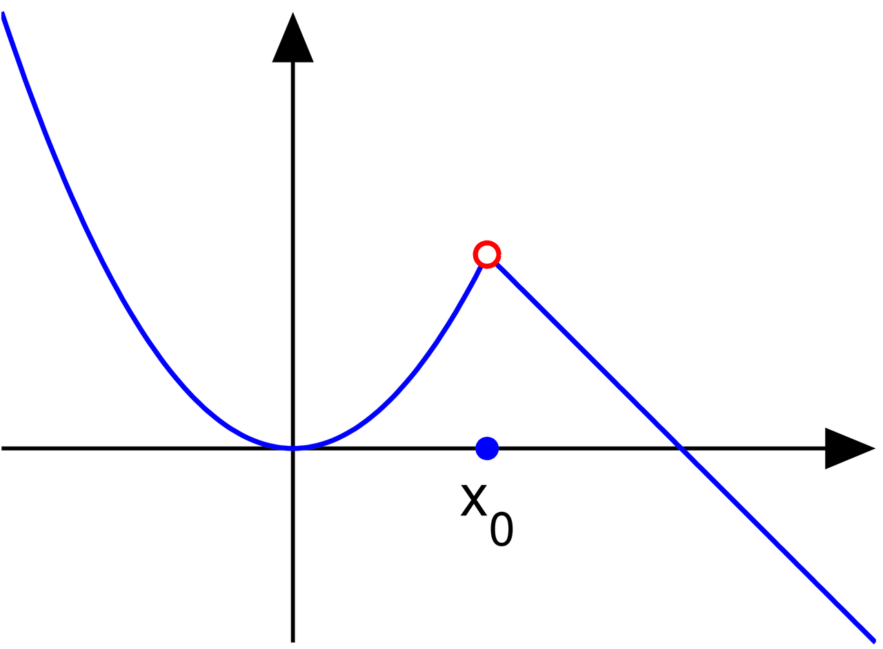
ある点における関数の振動は、これらの不連続性を次のように定量化します。

• 除去可能な不連続性では、関数の値がずれる距離が振動です。
• ジャンプ不連続では、ジャンプのサイズが振動です（その点の値が2つの側のこれらの限界値の間にあると仮定します）。
• 本質的な不連続性（無限不連続性とも呼ばれる）において、振動は限界が存在しないことを測定します。

特別なケースとして、関数が無限大またはマイナス無限大に発散する場合があり、その場合には振動は定義されません (拡張実数では、これは除去可能な不連続性です)。

分類

以下のそれぞれについて、が不連続となる点の近傍で定義された実変数の実数値関数 を考えます。 ${\displaystyle f}$ ${\displaystyle x,}$ ${\displaystyle x_{0}}$ ${\displaystyle f}$

除去可能な不連続性

例1の関数、除去可能な不連続性

区分関数 を考える $${\displaystyle f(x)={\begin{cases}x^{2}&{\text{ for }}x<1\\0&{\text{ for }}x=1\\2-x&{\text{ for }}x>1\end{cases}}}$$

問題は、除去可能な不連続性です。この種の不連続性については、次のようになります。 ${\displaystyle x_{0}=1}$

負方向からの片側極限：と正方向からの片側極限： は両方ともに存在し、有限であり、 に等しい。言い換えれば、2つの片側極限が存在し、 が等しいので、が に近づくときの の極限が存在し、 はこの同じ値に等しい。 の実際の値が に等しくない場合、はと呼ばれる。 $${\displaystyle L^{-}=\lim _{x\to x_{0}^{-}}f(x)}$$ $${\displaystyle L^{+}=\lim _{x\to x_{0}^{+}}f(x)}$$ ${\displaystyle x_{0}}$ ${\displaystyle L=L^{-}=L^{+}.}$ ${\displaystyle L}$ ${\displaystyle f(x)}$ ${\displaystyle x}$ ${\displaystyle x_{0}}$ ${\displaystyle f\left(x_{0}\right)}$ ${\displaystyle L,}$ ${\displaystyle x_{0}}$除去可能な不連続性。この不連続性を除去すると、連続により正確には、関数は連続である。 ${\displaystyle f}$ ${\displaystyle x_{0},}$ $${\displaystyle g(x)={\begin{cases}f(x)&x\neq x_{0}\\L&x=x_{0}\end{cases}}}$$ ${\displaystyle x=x_{0}.}$

除去可能な不連続性という用語は、両方向の極限が存在して等しいが、点^{[a]では関数が}定義されていない、除去可能な特異点を含むように拡大解釈されることがあります。関数の連続性と不連続性は、関数の定義域内の点に対してのみ定義される概念であるため、この用法は用語の乱用です。 ${\displaystyle x_{0}.}$

ジャンプの不連続性

例2の関数、ジャンプ不連続

機能について考える $${\displaystyle f(x)={\begin{cases}x^{2}&{\mbox{ for }}x<1\\0&{\mbox{ for }}x=1\\2-(x-1)^{2}&{\mbox{ for }}x>1\end{cases}}}$$

さて、ポイントは ${\displaystyle x_{0}=1}$ジャンプ不連続。

この場合、片側極限、およびが存在し、有限であるものの等しくないため、単一の極限は存在しません。したがって、極限は存在しません。したがって、はジャンプ不連続、ステップ不連続、または第一種不連続と呼ばれます。このタイプの不連続では、関数は任意の値を取ることができます。 ${\displaystyle L^{-}}$ ${\displaystyle L^{+}}$ ${\displaystyle L^{-}\neq L^{+},}$ ${\displaystyle L}$ ${\displaystyle x_{0}}$ ${\displaystyle f}$ ${\displaystyle x_{0}.}$

本質的な不連続性

例3の関数は、本質的な不連続性である

本質的な不連続性の場合、2 つの片側極限のうち少なくとも 1 つは に存在しません。(片側極限の 1 つまたは両方が になる可能性があることに注意してください)。 ${\displaystyle \mathbb {R} }$ ${\displaystyle \pm \infty }$

機能について考える $${\displaystyle f(x)={\begin{cases}\sin {\frac {5}{x-1}}&{\text{ for }}x<1\\0&{\text{ for }}x=1\\{\frac {1}{x-1}}&{\text{ for }}x>1.\end{cases}}}$$

さて、ポイントは ${\displaystyle x_{0}=1}$本質的な不連続性。

この例では、 と はどちらも には 存在しないため、本質的不連続性の条件を満たしています。 は本質的不連続性、無限不連続性、または第二種不連続性です。（これは、複素変数の関数を研究する際によく使用される本質的特異点とは異なります）。 ${\displaystyle L^{-}}$ ${\displaystyle L^{+}}$ ${\displaystyle \mathbb {R} }$ ${\displaystyle x_{0}}$

関数の不連続点を数える

が区間上で定義された関数であると仮定すると、における不連続点すべての集合を で表す。によって、 で除去可能な不連続点を持つすべての集合を意味する。同様に、でジャンプ不連続点を持つすべての集合を表す。で本質的な不連続点を持つすべての集合はで表す。もちろん、 ${\displaystyle f}$ ${\displaystyle I\subseteq \mathbb {R} ,}$ ${\displaystyle D}$ ${\displaystyle f}$ ${\displaystyle I.}$ ${\displaystyle R}$ ${\displaystyle x_{0}\in I}$ ${\displaystyle f}$ ${\displaystyle x_{0}.}$ ${\displaystyle J}$ ${\displaystyle x_{0}\in I}$ ${\displaystyle f}$ ${\displaystyle x_{0}.}$ ${\displaystyle x_{0}\in I}$ ${\displaystyle f}$ ${\displaystyle x_{0}}$ ${\displaystyle E.}$ ${\displaystyle D=R\cup J\cup E.}$

このセットの次の 2 つの特性は文献で関連しています。 ${\displaystyle D}$

• 集合は集合である。関数が連続となる点の集合は常に集合である（^[2]を参照）。 ${\displaystyle D}$ ${\displaystyle F_{\sigma }}$ ${\displaystyle G_{\delta }}$
• 区間 が単調である場合、 は最大でも可算であり、これがフローダの定理です。 ${\displaystyle I,}$ ${\displaystyle f}$ ${\displaystyle D}$ ${\displaystyle D=J.}$

トム・アポストル^[3]は、上記の分類に部分的に従い、除去可能不連続性とジャンプ不連続性のみを考察している。彼の目的は単調関数の不連続性を研究し、主にフロダの定理を証明することである。同じ目的で、ウォルター・ルーディン^[4]とカール・R・ストロムバーグ^[5]も、異なる用語を用いて除去可能不連続性とジャンプ不連続性を研究している。しかし、さらに両著者とも、 は常に可算集合であると述べている（^{[6] [7]}を参照）。 ${\displaystyle R\cup J}$

本質的不連続性という用語は、1889年には既に数学的な文脈で使用されていた証拠がある。^[8]しかし、この用語が数学的な定義と併せて使用された最も古い例は、ジョン・クリッパートの著作であると思われる。^[9]その著作の中で、クリッパートは本質的不連続性自体を、以下の3つの集合に細分化して分類した。 ${\displaystyle E}$

$${\displaystyle E_{1}=\left\{x_{0}\in I:\lim _{x\to x_{0}^{-}}f(x){\text{ and }}\lim _{x\to x_{0}^{+}}f(x){\text{ do not exist in }}\mathbb {R} \right\},}$$ $${\displaystyle E_{2}=\left\{x_{0}\in I:\ \lim _{x\to x_{0}^{-}}f(x){\text{ exists in }}\mathbb {R} {\text{ and }}\lim _{x\to x_{0}^{+}}f(x){\text{ does not exist in }}\mathbb {R} \right\},}$$ $${\displaystyle E_{3}=\left\{x_{0}\in I:\ \lim _{x\to x_{0}^{-}}f(x){\text{ does not exist in }}\mathbb {R} {\text{ and }}\lim _{x\to x_{0}^{+}}f(x){\text{ exists in }}\mathbb {R} \right\}.}$$

もちろん、Wheneverは第一種の本質的不連続性と呼ばれます。Anyは第二種の本質的不連続性と呼ばれます。そこで彼は、次のように述べることで、可算であるという性質を失うことなく集合を拡大します。 ${\displaystyle E=E_{1}\cup E_{2}\cup E_{3}.}$ ${\displaystyle x_{0}\in E_{1},}$ ${\displaystyle x_{0}}$ ${\displaystyle x_{0}\in E_{2}\cup E_{3}}$ ${\displaystyle R\cup J}$

• この集合は可算です。 ${\displaystyle R\cup J\cup E_{2}\cup E_{3}}$

ルベーグの定理の書き換え

およびが有界関数のとき、のリーマン積分可能性に関する集合 の重要性はよく知られています。実際、ルベーグの定理 (ルベーグ-ヴィタリの定理とも呼ばれる) によれば、が 上でリーマン積分可能であるのは、がルベーグ測度が 0 である集合である場合のみです。 ${\displaystyle I=[a,b]}$ ${\displaystyle f}$ ${\displaystyle D}$ ${\displaystyle f.}$ ${\displaystyle f}$ ${\displaystyle I=[a,b]}$ ${\displaystyle D}$

この定理では、有界関数がリーマン積分可能であるという障害に対して、あらゆる種類の不連続性が同等の重みを持つように思われる。可算集合はルベーグ測度零の集合であり、ルベーグ測度零を持つ集合の可算和もやはりルベーグ測度零の集合であるため、これは当てはまらないことが分かる。実際、集合内の不連続性は、リーマン積分可能性に関して全く中立である。この目的のための主要な不連続性は第一種の本質的不連続性であり、したがってルベーグ＝ヴィタリの定理は次のように書き直すことができる。 ${\displaystyle f}$ ${\displaystyle [a,b].}$ ${\displaystyle R\cup J\cup E_{2}\cup E_{3}}$ ${\displaystyle f.}$

• 有界関数は、第 1 種のすべての本質的不連続性の対応集合がルベーグ測度 0 を持つ場合のみ、上でリーマン積分可能です。 ${\displaystyle f,}$ ${\displaystyle [a,b]}$ ${\displaystyle E_{1}}$ ${\displaystyle f}$

の場合は、有界関数のリーマン積分可能性に関する次のようなよく知られた古典的な補完状況に対応します。 ${\displaystyle E_{1}=\varnothing }$ ${\displaystyle f:[a,b]\to \mathbb {R} }$

• の各点で右極限を持つ場合、はリーマン積分可能である（^[10]を参照） ${\displaystyle f}$ ${\displaystyle [a,b[}$ ${\displaystyle f}$ ${\displaystyle [a,b]}$
• の各点で左極限を持つ場合、リーマン積分は ${\displaystyle f}$ ${\displaystyle ]a,b]}$ ${\displaystyle f}$ ${\displaystyle [a,b].}$
• が上の規制関数であるとき、リーマン積分は上で ${\displaystyle f}$ ${\displaystyle [a,b]}$ ${\displaystyle f}$ ${\displaystyle [a,b].}$

例

トーマ関数は、すべての非零有理点において不連続であるが、すべての無理点において連続である。これらの不連続性はすべて除去可能であることは容易に理解できる。最初の段落で述べたように、すべての有理点において連続であるが、すべての無理点において不連続である関数は存在しない。

有理数の指示関数（ディリクレ関数とも呼ばれる）は、あらゆる点で不連続である。これらの不連続性はすべて、第一種の性質を持つ。

ここで、三元カントール集合 とその指示関数（特性関数） を考えてみましょう。カントール集合を​​構成する一つの方法は、次のように与えられます。ここで、集合は再帰法によって次のように得られます。 ${\displaystyle {\mathcal {C}}\subset [0,1]}$ $${\displaystyle \mathbf {1} _{\mathcal {C}}(x)={\begin{cases}1&x\in {\mathcal {C}}\\0&x\in [0,1]\setminus {\mathcal {C}}.\end{cases}}}$$ ${\displaystyle {\mathcal {C}}}$ ${\textstyle {\mathcal {C}}:=\bigcap _{n=0}^{\infty }C_{n}}$ ${\displaystyle C_{n}}$ $${\displaystyle C_{n}={\frac {C_{n-1}}{3}}\cup \left({\frac {2}{3}}+{\frac {C_{n-1}}{3}}\right){\text{ for }}n\geq 1,{\text{ and }}C_{0}=[0,1].}$$

関数の不連続性を考慮して、点を仮定してみましょう。 ${\displaystyle \mathbf {1} _{\mathcal {C}}(x),}$ ${\displaystyle x_{0}\not \in {\mathcal {C}}.}$

したがって、の定式化に用いられる集合が存在し、これは を含まない。つまり、は の構築で除去された開区間の1つに属する。このように、は の点を含まない近傍を持つ（言い換えれば、は閉集合であり、 に対するその補集合は開集合であることを考慮すると、同じ結論が導かれる）。したがって、はのある近傍においてのみ値0をとる。したがって、 は で連続である。 ${\displaystyle C_{n},}$ ${\displaystyle {\mathcal {C}}}$ ${\displaystyle x_{0}.}$ ${\displaystyle x_{0}}$ ${\displaystyle C_{n}.}$ ${\displaystyle x_{0}}$ ${\displaystyle {\mathcal {C}}.}$ ${\displaystyle {\mathcal {C}}}$ ${\displaystyle [0,1]}$ ${\displaystyle \mathbf {1} _{\mathcal {C}}}$ ${\displaystyle x_{0}.}$ ${\displaystyle \mathbf {1} _{\mathcal {C}}}$ ${\displaystyle x_{0}.}$

これは、区間 上の のすべての不連続性の集合がのサブセットであることを意味します。はルベーグ測度がゼロの不可算集合であるため、 もルベーグ測度集合であり、したがってルベーグ-ヴィタリの定理に関して、はリーマン積分関数です。 ${\displaystyle D}$ ${\displaystyle \mathbf {1} _{\mathcal {C}}}$ ${\displaystyle [0,1]}$ ${\displaystyle {\mathcal {C}}.}$ ${\displaystyle {\mathcal {C}}}$ ${\displaystyle D}$ ${\displaystyle \mathbf {1} _{\mathcal {C}}}$

より正確には、 である。実際、はどこにも稠密でない集合なので、の近傍は には含まれない。このように、 の任意の近傍はの点とに含まれない点を含む。関数 に関して言えば、これはと がどちらも存在しないことを意味する。つまり、 である。ここで、前と同様に、によって関数の第一種 のすべての本質的不連続の集合を表す。明らかに ${\displaystyle D={\mathcal {C}}.}$ ${\displaystyle {\mathcal {C}}}$ ${\displaystyle x_{0}\in {\mathcal {C}}}$ ${\displaystyle \left(x_{0}-\varepsilon ,x_{0}+\varepsilon \right)}$ ${\displaystyle x_{0},}$ ${\displaystyle {\mathcal {C}}.}$ ${\displaystyle x_{0}\in {\mathcal {C}}}$ ${\displaystyle {\mathcal {C}}}$ ${\displaystyle {\mathcal {C}}.}$ ${\displaystyle \mathbf {1} _{\mathcal {C}}}$ ${\textstyle \lim _{x\to x_{0}^{-}}\mathbf {1} _{\mathcal {C}}(x)}$ ${\textstyle \lim _{x\to x_{0}^{+}}1_{\mathcal {C}}(x)}$ ${\displaystyle D=E_{1},}$ ${\displaystyle E_{1},}$ ${\displaystyle \mathbf {1} _{\mathcal {C}}.}$ ${\textstyle \int _{0}^{1}\mathbf {1} _{\mathcal {C}}(x)dx=0.}$

微分の不連続性

開区間を とし、が 上で微分可能で がの導関数であるとする。つまり、任意の に対して となる。ダルブーの定理によれば、導関数は中間値の性質を満たす。もちろん、関数は区間 上で連続になることもあり、その場合にはボルザノの定理も適用される。ボルザノの定理は、すべての連続関数が中間値の性質を満たすことを主張していることを思い出してほしい。一方、逆は偽である。ダルブーの定理は が連続であると仮定しておらず、中間値の性質はが 上で連続であることを意味しない。 ${\displaystyle I\subseteq \mathbb {R} }$ ${\displaystyle F:I\to \mathbb {R} }$ ${\displaystyle I,}$ ${\displaystyle f:I\to \mathbb {R} }$ ${\displaystyle F.}$ ${\displaystyle F'(x)=f(x)}$ ${\displaystyle x\in I}$ ${\displaystyle f:I\to \mathbb {R} }$ ${\displaystyle f}$ ${\displaystyle I,}$ ${\displaystyle f}$ ${\displaystyle f}$ ${\displaystyle I.}$

しかしながら、ダルブーの定理は、 がどのような不連続性を持ち得るかという点に直接的な影響を及ぼします。実際、が の不連続点である場合、 は必然的にの本質的不連続点となります。^[11]これは特に、以下の2つの状況は発生しないことを意味します。 ${\displaystyle f}$ ${\displaystyle x_{0}\in I}$ ${\displaystyle f}$ ${\displaystyle x_{0}}$ ${\displaystyle f}$

1. ${\displaystyle x_{0}}$は の除去可能な不連続点です。 ${\displaystyle f}$
2. ${\displaystyle x_{0}}$は のジャンプ不連続です。 ${\displaystyle f}$

さらに、他の2つの状況を除外する必要があります（ジョン・クリッパート^[12]を参照）。

3. ${\displaystyle \lim _{x\to x_{0}^{-}}f(x)=\pm \infty .}$
4. ${\displaystyle \lim _{x\to x_{0}^{+}}f(x)=\pm \infty .}$

条件 (i)、(ii)、(iii)、(iv) のいずれかが に対して満たされる場合は常に、 は区間 上で原始微分、を持たないと結論付けることができることに注意してください。 ${\displaystyle x_{0}\in I}$ ${\displaystyle f}$ ${\displaystyle F}$ ${\displaystyle I}$

一方、任意の関数に関して新しいタイプの不連続性を導入することができる。関数 の本質的不連続性 は、の基本的な本質的不連続性であると言われる。 ${\displaystyle f:I\to \mathbb {R} }$ ${\displaystyle x_{0}\in I}$ ${\displaystyle f}$ ${\displaystyle f}$

$${\displaystyle \lim _{x\to x_{0}^{-}}f(x)\neq \pm \infty }$$そして $${\displaystyle \lim _{x\to x_{0}^{+}}f(x)\neq \pm \infty .}$$

したがって、が微分関数 の不連続性である場合、 は必然的にの基本的な本質的不連続性です。 ${\displaystyle x_{0}\in I}$ ${\displaystyle f:I\to \mathbb {R} }$ ${\displaystyle x_{0}}$ ${\displaystyle f}$

また、およびが有界関数であるとき 、ルベーグの定理の仮定にあるように、すべての に対して が成り立つことにも注意してください。 したがって、の任意の本質的不連続性は基本的な不連続性です。 ${\displaystyle I=[a,b]}$ ${\displaystyle f:I\to \mathbb {R} }$ ${\displaystyle x_{0}\in (a,b)}$ $${\displaystyle \lim _{x\to x_{0}^{\pm }}f(x)\neq \pm \infty ,}$$ $${\displaystyle \lim _{x\to a^{+}}f(x)\neq \pm \infty ,}$$ $${\displaystyle \lim _{x\to b^{-}}f(x)\neq \pm \infty .}$$ ${\displaystyle f}$

参照

• 除去可能な特異点 – 正則関数上の未定義の点であり、正則化できる
• 数学的特異点 – 数学的対象が不規則に振る舞う点Pages displaying short descriptions of redirect targets
• 連続性による拡張 – 位相空間の性質
• 滑らかさ – 関数の導関数の数（数学）
  • 幾何学的連続性 - 関数の導関数の数（数学）Pages displaying short descriptions of redirect targets
  • 媒介変数連続性 – 関数の導関数の数（数学）Pages displaying short descriptions of redirect targets

注記

1. 例えば、Mathwordsの定義の最後の文を参照してください。^[1]

参考文献

1. 「Mathwords: 除去可能な不連続性」.
2. ストロンバーグ、カール・R. (2015). 『古典実解析入門』アメリカ数学会. p. 120. 例3 (c). ISBN 978-1-4704-2544-9。
3. アポストル、トム (1974). 『数学的解析』（第2版）. アディソン＆ウェスレー. p. 92, sec. 4.22, sec. 4.23 and Ex. 4.63. ISBN 0-201-00288-4。
4. ウォルター・ルディン (1976). 『数学解析の原理』（第3版）. マグロウヒル. pp. 94, 定義4.26, 定義4.29, 定義4.30. ISBN 0-07-085613-3。
5. Stromberg, Karl R.前掲書. p. 128, 定義 3.87, 解釈 3.90.
6. ウォルター・ルディン。前掲書。100ページ、資料17。
7. ストロンバーグ、カールR.前掲書. p. 131、Ex. 3。
8. ホイットニー、ウィリアム・ドワイト (1889). 『センチュリー辞典：英語百科事典』第2巻. ロンドンおよびニューヨーク: T. フィッシャー・アンウィンおよびセンチュリー社. p. 1652. ISBN 97813341539522008年12月16日にオリジナルからアーカイブされました。本質的不連続とは、関数の値が完全に不確定となる不連続のことです。 {{cite book}}: ISBN / Date incompatibility (help)
9. クリッパート, ジョン (1989年2月). 「上級微積分学：区間領域における実数値関数の不連続点の計算」.数学マガジン. 62 : 43–48 . doi :10.1080/0025570X.1989.11977410.
10. Metzler, RC (1971). 「リーマン積分可能性について」 .アメリカ数学月刊誌. 78 (10): 1129– 1131. doi :10.1080/00029890.1971.11992961.
11. ルディン、ウォルター。前掲書。pp . 109、系。
12. Klippert, John (2000). 「導関数の不連続性について」 .国際数学教育科学技術誌. 31:S2: 282– 287. Bibcode :2000IJMES..31..282K. doi :10.1080/00207390050032252.

出典

• マリク, SC; アローラ, サビタ (1992). 『数学的解析』（第2版）. ニューヨーク: Wiley. ISBN 0-470-21858-4。{{cite book}}: CS1 maint: publisher location (link)

外部リンク

• 「不連続」。PlanetMath。
• 「不連続性」、Ed Pegg, Jr.著、The Wolfram Demonstrations Project、2007 年。
• ワイスタイン、エリック・W.「不連続性」。MathWorld。
• Kudryavtsev, LD (2001) [1994]. 「不連続点」.数学百科事典. EMS Press .

Retrieved from "https://en.wikipedia.org/w/index.php?title=Classification_of_discontinuities&oldid=1321978961"