発散定理

Theorem in calculus which relates the flux of closed surfaces to divergence over their volume

ベクトル解析において、発散定理はガウスの定理やオストログラツキーの定理とも呼ばれ、^[1]閉じた表面を通るベクトル場の流束と、閉じた体積内の場 の発散を関連付ける定理です。

より正確には、発散定理とは、閉曲面上のベクトル場の面積分（面を通る「フラックス」と呼ばれる）が、その面に囲まれた領域における発散の体積積分に等しいことを述べています。直感的に言えば、これは「ある領域における場のすべての発生源（シンクは負の発生源とみなす）の総和が、その領域から出る正味のフラックスを与える」ということを述べています。

発散定理は、物理学と工学の数学、特に静電気学と流体力学において重要な結果です。これらの分野では、通常3次元に適用されますが、任意の次元数に一般化できます。1次元では、微積分学の基本定理に相当し、2次元ではグリーンの定理に相当します。

液体の流れを用いた説明

ベクトル場は、気体や液体などの流体の速度場の例を用いて説明されることが多い。移動する液体は、各点において速度（速さと方向）を持ち、これはベクトルで表すことができるため、任意の瞬間における液体の速度はベクトル場を形成する。液体の体積を囲む液体内部の閉曲面Sを考えてみよう。任意の時点における液体の体積からの流束は、この表面を横切る流体の体積流量、すなわち表面上の速度の面積分に等しい。

液体は非圧縮性であるため、閉空間内の液体量は一定です。空間内に流入源や流入先がない場合、 Sからの液体の流出量はゼロです。液体が移動している場合、S面上のいくつかの点から空間内に流入し、他の点から空間外に流出する可能性がありますが、どの瞬間においても流入量と流出量は等しいため、空間外への液体の正味の流出量はゼロです。

しかし、液体の供給源が閉じた表面の内側にある場合（例えば、液体が導入されるパイプなど）、追加された液体は周囲の液体に圧力をかけ、あらゆる方向へ外向きの流れを引き起こします。これにより、表面Sを通る正味の外向きの流れが発生します。 Sを通る外向きの流束は、パイプからSに流入する流体の体積流量に等しくなります。同様に、 S内にシンクまたは排水口（例えば、液体を排出するパイプ）がある場合、液体の外圧によって、液体全体に排水口の位置に向かって内側に向いた速度が生じます。表面Sを通る液体の内向きの流量は、シンクによって除去される液体の速度に等しくなります。

S内に複数の液体の流入源と流入源がある場合、表面を通過するフラックスは、流入源から流入する液体の体積流量を合計し、流入源から流出する液体の体積流量を差し引くことで計算できます。流入源または流入源を通過する液体の体積流量（流入源を通過する液体の体積流量は負の符号で表されます）は、管口における速度場の発散に等しいため、 Sで囲まれた体積全体にわたる液体の発散を合計（積分）すると、Sを通過するフラックスの体積流量が得られます。これが発散定理です。^[2]

発散定理はあらゆる保存則に用いられ、すべてのシンクとソースの合計体積、つまり発散の体積積分が体積の境界を横切る正味の流れに等しいことを述べています。^[3]

数学的な記述

面法線nを持つ面S = ∂ Vで囲まれた領域V

Vが の部分集合であるとする（ n = 3の場合、 V は3次元空間の体積を表す）。V はコンパクトで、区分的に滑らかな境界S（ とも表記）を持つ。FがVの近傍で定義された連続微分可能ベクトル場である場合、次式が成り立つ：^{[4] [5]} ${\displaystyle \mathbb {R} ^{n}}$ ${\displaystyle \partial V=S}$

${\displaystyle \iiint _{V}\left(\mathbf {\nabla } \cdot \mathbf {F} \right)\,\mathrm {d} V=}$ ${\displaystyle \scriptstyle S}$ ${\displaystyle (\mathbf {F} \cdot \mathbf {\hat {n}} )\,\mathrm {d} S.}$

左辺は体積V上の体積積分であり、右辺は体積Vの境界上の面積分です。閉じた測定可能な集合は、外向きの法線によって方向付けられ、境界 上のほぼすべての点における外向きの単位法線 です。（はの略記として使用できます。）上記の直感的な説明で言えば、式の左辺は体積V内のソースの合計を表し、右辺は境界Sを横切る総流量を表します。 ${\displaystyle \partial V}$ ${\displaystyle \mathbf {\hat {n}} }$ ${\displaystyle \partial V}$ ${\displaystyle \mathrm {d} \mathbf {S} }$ ${\displaystyle \mathbf {n} \mathrm {d} S}$

非公式な派生

発散定理は、体積Vが別々の部分に分割された場合、元の体積から出るフラックスは、各構成体積から出るフラックスの代数和に等しいという事実から導かれます。^{[6] [7]} 新しいサブボリュームが元の体積の表面の一部ではなかった表面を持つという事実にもかかわらず、これは当てはまります。なぜなら、これらの表面は単に 2 つのサブボリューム間の仕切りであり、そこを通過するフラックスは 1 つのボリュームから他のボリュームに渡るだけなので、サブボリュームからのフラックスが合計されると打ち消されるからです。

2つのサブボリュームに分割されたボリューム。右側では、異なる表面からのフラックスを表示するために、2つのサブボリュームが分離されています。

図を見てください。閉じた有界体積Vは、面S ₃ (緑)によって2つの体積V ₁とV _{2に分割されています。各構成領域}V _iからの磁束Φ( V _i )は、その2つの面を通る磁束の合計に等しいため、2つの部分からの磁束の合計は

${\displaystyle \Phi (V_{\text{1}})+\Phi (V_{\text{2}})=\Phi _{\text{1}}+\Phi _{\text{31}}+\Phi _{\text{2}}+\Phi _{\text{32}}}$

ここで、Φ ₁とΦ _2は表面S ₁とS ₂から出る磁束、 Φ ₃₁は体積 1 からS ₃を通る磁束、 Φ _{32は体積 2 から}S ₃を通る磁束です。ポイントは、表面S ₃が両方の体積の表面の一部であるということです。法線ベクトルの「外向き」の方向は各体積で反対方向であるため、一方の体積から S ₃を通る磁束は、もう一方の体積から出る磁束の負の値に等しく、これら2つの磁束は合計で打ち消されます。 ${\displaystyle \mathbf {\hat {n}} }$

${\displaystyle \Phi _{\text{31}}=\iint _{S_{3}}\mathbf {F} \cdot \mathbf {\hat {n}} \;\mathrm {d} S=-\iint _{S_{3}}\mathbf {F} \cdot (-\mathbf {\hat {n}} )\;\mathrm {d} S=-\Phi _{\text{32}}}$

したがって：

${\displaystyle \Phi (V_{\text{1}})+\Phi (V_{\text{2}})=\Phi _{\text{1}}+\Phi _{\text{2}}}$

面S ₁とS ₂の和はS

${\displaystyle \Phi (V_{\text{1}})+\Phi (V_{\text{2}})=\Phi (V)}$

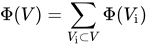
体積は任意の数のサブボリュームに分割することができ、Vからのフラックスは各サブボリュームからのフラックスの合計に等しくなります。これは、緑色の表面を通るフラックスが合計で打ち消されるためです。(b)では、体積がわずかに離れており、緑色の区画がそれぞれ隣接する2つの体積の境界の一部であることを示しています。

この原理は、図に示すように、任意の数の部分に分割された体積に適用されます。^{[7]各内部区画}（緑色の面） の積分は、隣接する2つの体積のフラックスにおいて反対の符号で現れるため、それらは打ち消され、フラックスへの寄与は外部表面（灰色）の積分のみとなります。すべての構成体積の外面は元の表面積に等しいためです。

${\displaystyle \Phi (V)=\sum _{V_{\text{i}}\subset V}\Phi (V_{\text{i}})}$

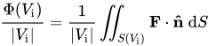
体積が小さな部分に分割されるにつれて、各体積からのフラックスと体積の比率は近づきます。 ${\displaystyle \Phi (V_{\text{i}})}$ ${\displaystyle |V_{\text{i}}|}$ ${\displaystyle \operatorname {div} \mathbf {F} }$

各体積からの流束Φは、表面上の ベクトル場F ( x )の面積分である。

${\displaystyle \iint _{S(V)}\mathbf {F} \cdot \mathbf {\hat {n}} \;\mathrm {d} S=\sum _{V_{\text{i}}\subset V}\iint _{S(V_{\text{i}})}\mathbf {F} \cdot \mathbf {\hat {n}} \;\mathrm {d} S}$

目標は、元の体積を無限に多くの微小体積に分割することです。体積がどんどん小さな部分に分割されるにつれて、右辺の表面積積分、つまり各部分体積からのフラックスは、表面積S ( V _i )がゼロに近づくため、ゼロに近づきます。しかし、発散の定義から、フラックスと体積の比、つまり以下の括弧内の部分は、一般にはゼロにならず、体積がゼロに近づくにつれて発散div F^{に近づきます。 [7]} ${\displaystyle {\frac {\Phi (V_{\text{i}})}{|V_{\text{i}}|}}={\frac {1}{|V_{\text{i}}|}}\iint _{S(V_{\text{i}})}\mathbf {F} \cdot \mathbf {\hat {n}} \;\mathrm {d} S}$

${\displaystyle \iint _{S(V)}\mathbf {F} \cdot \mathbf {\hat {n}} \;\mathrm {d} S=\sum _{V_{\text{i}}\subset V}\left({\frac {1}{|V_{\text{i}}|}}\iint _{S(V_{\text{i}})}\mathbf {F} \cdot \mathbf {\hat {n}} \;\mathrm {d} S\right)|V_{\text{i}}|}$

ベクトル場F ( x )が連続微分を持つ限り、上記の和は体積が無限に小さな増分に分割された極限でも成立する。

${\displaystyle \iint _{S(V)}\mathbf {F} \cdot \mathbf {\hat {n}} \;\mathrm {d} S=\lim _{|V_{\text{i}}|\to 0}\sum _{V_{\text{i}}\subset V}\left({\frac {1}{|V_{\text{i}}|}}\iint _{S(V_{\text{i}})}\mathbf {F} \cdot \mathbf {\hat {n}} \;\mathrm {d} S\right)|V_{\text{i}}|}$

体積がゼロに近づくと、無限小のdVとなり、括弧内の部分は発散となり、その合計はVについての体積積分となる。 ${\displaystyle |V_{\text{i}}|}$

${\displaystyle \;\iint _{S(V)}\mathbf {F} \cdot \mathbf {\hat {n}} \;\mathrm {d} S=\iiint _{V}\operatorname {div} \mathbf {F} \;\mathrm {d} V\;}$

この導出は座標フリーであるため、発散は使用される座標に依存しないことがわかります。

証明

ユークリッド空間の有界開集合の場合

以下を証明します。^[要引用]

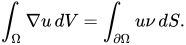
定理—が開状態で、境界が で有界であるとする。が の開近傍、つまり上にある場合、各 に対して、はへの外向きの単位法線ベクトルである。同様に、 ${\displaystyle \Omega \subset \mathbb {R} ^{n}}$ ${\displaystyle C^{1}}$ ${\displaystyle u}$ ${\displaystyle C^{1}}$ ${\displaystyle O}$ ${\displaystyle {\overline {\Omega }}}$ ${\displaystyle u\in C^{1}(O)}$ ${\displaystyle i\in \{1,\dots ,n\}}$ $${\displaystyle \int _{\Omega }u_{x_{i}}\,dV=\int _{\partial \Omega }u\nu _{i}\,dS,}$$ ${\displaystyle \nu :\partial \Omega \to \mathbb {R} ^{n}}$ ${\displaystyle \partial \Omega }$ $${\displaystyle \int _{\Omega }\nabla u\,dV=\int _{\partial \Omega }u\nu \,dS.}$$

定理の証明^[8]

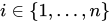
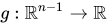
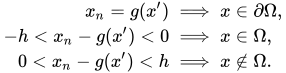
1. 最初のステップは、 の場合に帰着することです。上でとなるものを選びます。上でかつ となることに注意してください。したがって、 の定理を証明すれば十分です。したがって、 と仮定できます。 ${\displaystyle u\in C_{c}^{1}(\mathbb {R} ^{n})}$ ${\displaystyle \phi \in C_{c}^{\infty }(O)}$ ${\displaystyle \phi =1}$ ${\displaystyle {\overline {\Omega }}}$ ${\displaystyle \phi u\in C_{c}^{1}(O)\subset C_{c}^{1}(\mathbb {R} ^{n})}$ ${\displaystyle \phi u=u}$ ${\displaystyle {\overline {\Omega }}}$ ${\displaystyle \phi u}$ ${\displaystyle u\in C_{c}^{1}(\mathbb {R} ^{n})}$
2. を任意とします。境界を持つという仮定は、の開近傍が存在し、はこのグラフの片側に関数のグラフであることを意味します。より正確には、 を平行移動および回転させた後、とおよび関数 が存在し、 という表記で ${\displaystyle x_{0}\in \partial \Omega }$ ${\displaystyle {\overline {\Omega }}}$ ${\displaystyle C^{1}}$ ${\displaystyle U}$ ${\displaystyle x_{0}}$ ${\displaystyle \mathbb {R} ^{n}}$ ${\displaystyle \partial \Omega \cap U}$ ${\displaystyle C^{1}}$ ${\displaystyle \Omega \cap U}$ ${\displaystyle \Omega }$ ${\displaystyle r>0}$ ${\displaystyle h>0}$ ${\displaystyle C^{1}}$ ${\displaystyle g:\mathbb {R} ^{n-1}\to \mathbb {R} }$

   $${\displaystyle x'=(x_{1},\dots ,x_{n-1}),}$$およびに対して が成り立ち、 $${\displaystyle U=\{x\in \mathbb {R} ^{n}:|x'|<r{\text{ and }}|x_{n}-g(x')|<h\}}$$ ${\displaystyle x\in U}$ $${\displaystyle {\begin{aligned}x_{n}=g(x')&\implies x\in \partial \Omega ,\\-h<x_{n}-g(x')<0&\implies x\in \Omega ,\\0<x_{n}-g(x')<h&\implies x\notin \Omega .\\\end{aligned}}}$$

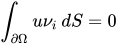
   はコンパクトなので、上記の形式の有限個の近傍で覆うことができます。は の開被覆であることに注意してください。この被覆に従属する1 の分割を使用することで、 がでコンパクトな台を持つか、何らかの でコンパクトな台を持つ場合の定理を証明すれば十分です。がでコンパクトな台を持つ場合、微積分学の基本定理により、すべての に対して が成り立ち、はの近傍で消えるためです。したがって、でコンパクトな台を持つ に対して定理が成り立ちます。したがって、が何らかの でコンパクトな台を持つ場合にまで簡約されました。 ${\displaystyle \partial \Omega }$ ${\displaystyle \partial \Omega }$ ${\displaystyle U_{1},\dots ,U_{N}}$ ${\displaystyle \{\Omega ,U_{1},\dots ,U_{N}\}}$ ${\displaystyle {\overline {\Omega }}=\Omega \cup \partial \Omega }$ ${\displaystyle C^{\infty }}$ ${\displaystyle u}$ ${\displaystyle \Omega }$ ${\displaystyle u}$ ${\displaystyle U_{j}}$ ${\displaystyle u}$ ${\displaystyle \Omega }$ ${\displaystyle i\in \{1,\dots ,n\}}$ ${\displaystyle \int _{\Omega }u_{x_{i}}\,dV=\int _{\mathbb {R} ^{n}}u_{x_{i}}\,dV=\int _{\mathbb {R} ^{n-1}}\int _{-\infty }^{\infty }u_{x_{i}}(x)\,dx_{i}\,dx'=0}$ ${\displaystyle \int _{\partial \Omega }u\nu _{i}\,dS=0}$ ${\displaystyle u}$ ${\displaystyle \partial \Omega }$ ${\displaystyle u}$ ${\displaystyle \Omega }$ ${\displaystyle u}$ ${\displaystyle U_{j}}$
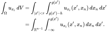
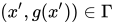
3. したがって、 はある においてコンパクト サポートを持つと仮定します。最後のステップは、直接計算によって定理が正しいことを示すことです。表記を に変更し、 を記述するために使用した (2) の表記を持ち込みます。これは、 を回転および平行移動したことを意味することに注意してください。定理は座標の回転および平行移動に対して不変であるため、これは有効な簡約です。 に対して、に対して であるため、各 に対して が成り立ちます。に対して、微積分の基本定理により、 が成り立ちます。ここで、 を固定します。が によって定義されることに注意してください。連鎖律により、しかし、 はコンパクト サポートを持つため、まず を 積分して を導き出すことができます。したがって をまとめると、 に対して は次のようになります。のグラフに対する点における外向きの単位法線はであり、面要素は によって与えられることを思い出してください。したがってこれで証明は完了です。 ${\displaystyle u}$ ${\displaystyle U_{j}}$ ${\displaystyle U=U_{j}}$ ${\displaystyle U}$ ${\displaystyle \Omega }$ ${\displaystyle u(x)=0}$ ${\displaystyle |x'|\geq r}$ ${\displaystyle |x_{n}-g(x')|\geq h}$ ${\displaystyle i\in \{1,\dots ,n\}}$ $${\displaystyle {\begin{aligned}\int _{\Omega }u_{x_{i}}\,dV&=\int _{|x'|<r}\int _{g(x')-h}^{g(x')}u_{x_{i}}(x',x_{n})\,dx_{n}\,dx'\\&=\int _{\mathbb {R} ^{n-1}}\int _{-\infty }^{g(x')}u_{x_{i}}(x',x_{n})\,dx_{n}\,dx'.\end{aligned}}}$$ ${\displaystyle i=n}$ $${\displaystyle \int _{\mathbb {R} ^{n-1}}\int _{-\infty }^{g(x')}u_{x_{n}}(x',x_{n})\,dx_{n}\,dx'=\int _{\mathbb {R} ^{n-1}}u(x',g(x'))\,dx'.}$$ ${\displaystyle i\in \{1,\dots ,n-1\}}$ $${\displaystyle \int _{\mathbb {R} ^{n-1}}\int _{-\infty }^{g(x')}u_{x_{i}}(x',x_{n})\,dx_{n}\,dx'=\int _{\mathbb {R} ^{n-1}}\int _{-\infty }^{0}u_{x_{i}}(x',g(x')+s)\,ds\,dx'}$$ ${\displaystyle v:\mathbb {R} ^{n}\to \mathbb {R} }$ ${\displaystyle v(x',s)=u(x',g(x')+s)}$ $${\displaystyle v_{x_{i}}(x',s)=u_{x_{i}}(x',g(x')+s)+u_{x_{n}}(x',g(x')+s)g_{x_{i}}(x').}$$ ${\displaystyle v}$ ${\displaystyle dx_{i}}$ $${\displaystyle \int _{\mathbb {R} ^{n-1}}\int _{-\infty }^{0}v_{x_{i}}(x',s)\,ds\,dx'=0.}$$ $${\displaystyle {\begin{aligned}\int _{\mathbb {R} ^{n-1}}\int _{-\infty }^{0}u_{x_{i}}(x',g(x')+s)\,ds\,dx'&=\int _{\mathbb {R} ^{n-1}}\int _{-\infty }^{0}-u_{x_{n}}(x',g(x')+s)g_{x_{i}}(x')\,ds\,dx'\\&=\int _{\mathbb {R} ^{n-1}}-u(x',g(x'))g_{x_{i}}(x')\,dx'.\end{aligned}}}$$ ${\displaystyle \nabla u=(u_{x_{1}},\dots ,u_{x_{n}})}$ $${\displaystyle \int _{\Omega }\nabla u\,dV=\int _{\mathbb {R} ^{n-1}}\int _{-\infty }^{g(x')}\nabla u\,dV=\int _{\mathbb {R} ^{n-1}}u(x',g(x'))(-\nabla g(x'),1)\,dx'.}$$ ${\displaystyle \Gamma }$ ${\displaystyle g}$ ${\displaystyle (x',g(x'))\in \Gamma }$ ${\displaystyle \nu (x',g(x'))={\frac {1}{\sqrt {1+|\nabla g(x')|^{2}}}}(-\nabla g(x'),1)}$ ${\displaystyle dS}$ ${\textstyle dS={\sqrt {1+|\nabla g(x')|^{2}}}\,dx'}$ $${\displaystyle \int _{\Omega }\nabla u\,dV=\int _{\partial \Omega }u\nu \,dS.}$$

境界を持つコンパクトリーマン多様体の場合

以下を証明します。^[要引用]

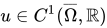
定理—を計量テンソルの境界を持つコンパクト多様体とします。を の多様体内部、 をの多様体境界 とします。を関数の内積、 をベクトルの内積とします。と を上のベクトル場とします。この 場合、への外向きの単位法線ベクトルはです。 ${\displaystyle {\overline {\Omega }}}$ ${\displaystyle C^{2}}$ ${\displaystyle C^{1}}$ ${\displaystyle g}$ ${\displaystyle \Omega }$ ${\displaystyle {\overline {\Omega }}}$ ${\displaystyle \partial \Omega }$ ${\displaystyle {\overline {\Omega }}}$ ${\displaystyle (\cdot ,\cdot )}$ ${\displaystyle L^{2}({\overline {\Omega }})}$ ${\displaystyle \langle \cdot ,\cdot \rangle }$ ${\displaystyle u\in C^{1}({\overline {\Omega }},\mathbb {R} )}$ ${\displaystyle X}$ ${\displaystyle C^{1}}$ ${\displaystyle {\overline {\Omega }}}$ $${\displaystyle (\operatorname {grad} u,X)=-(u,\operatorname {div} X)+\int _{\partial \Omega }u\langle X,N\rangle \,dS,}$$ ${\displaystyle N}$ ${\displaystyle \partial \Omega }$

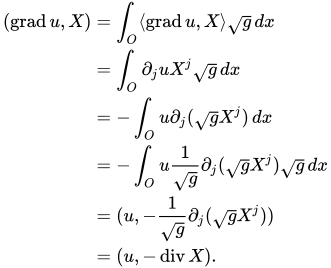
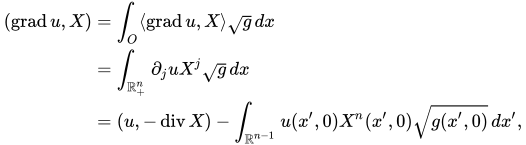
定理の証明。^[9]アインシュタインの総和規則を使用する。単位の分割を使用することにより、 と は座標パッチ においてコンパクトな台を持つと仮定できる。まず、パッチ が と素である場合を考える。すると はの開部分集合 と同一視され、部分積分では境界項は生成されない。最後の等式では、発散に対して Voss-Weyl 座標の式を使用したが、前述の恒等式を使用して を の形式的随伴として定義することもできる。次に、が と交差すると仮定する。すると は内の開集合 と同一視される。 とを に零拡張し、部分積分を実行して を得る 。ここで である。ベクトル場 の直線化定理の変形により、が における内向きの単位法線となるようにを選択できる。この場合は 上の体積要素であり、上式は次のようになる。これで証明は完了する。 ${\displaystyle u}$ ${\displaystyle X}$ ${\displaystyle O\subset {\overline {\Omega }}}$ ${\displaystyle \partial \Omega }$ ${\displaystyle O}$ ${\displaystyle \mathbb {R} ^{n}}$ $${\displaystyle {\begin{aligned}(\operatorname {grad} u,X)&=\int _{O}\langle \operatorname {grad} u,X\rangle {\sqrt {g}}\,dx\\&=\int _{O}\partial _{j}uX^{j}{\sqrt {g}}\,dx\\&=-\int _{O}u\partial _{j}({\sqrt {g}}X^{j})\,dx\\&=-\int _{O}u{\frac {1}{\sqrt {g}}}\partial _{j}({\sqrt {g}}X^{j}){\sqrt {g}}\,dx\\&=(u,-{\frac {1}{\sqrt {g}}}\partial _{j}({\sqrt {g}}X^{j}))\\&=(u,-\operatorname {div} X).\end{aligned}}}$$ ${\displaystyle -\operatorname {div} }$ ${\displaystyle \operatorname {grad} }$ ${\displaystyle O}$ ${\displaystyle \partial \Omega }$ ${\displaystyle O}$ ${\displaystyle \mathbb {R} _{+}^{n}=\{x\in \mathbb {R} ^{n}:x_{n}\geq 0\}}$ ${\displaystyle u}$ ${\displaystyle X}$ ${\displaystyle \mathbb {R} _{+}^{n}}$ $${\displaystyle {\begin{aligned}(\operatorname {grad} u,X)&=\int _{O}\langle \operatorname {grad} u,X\rangle {\sqrt {g}}\,dx\\&=\int _{\mathbb {R} _{+}^{n}}\partial _{j}uX^{j}{\sqrt {g}}\,dx\\&=(u,-\operatorname {div} X)-\int _{\mathbb {R} ^{n-1}}u(x',0)X^{n}(x',0){\sqrt {g(x',0)}}\,dx',\end{aligned}}}$$ ${\displaystyle dx'=dx_{1}\dots dx_{n-1}}$ ${\displaystyle O}$ ${\displaystyle {\frac {\partial }{\partial x_{n}}}}$ ${\displaystyle -N}$ ${\displaystyle \partial \Omega }$ ${\displaystyle {\sqrt {g(x',0)}}\,dx'={\sqrt {g_{\partial \Omega }(x')}}\,dx'=dS}$ ${\displaystyle \partial \Omega }$ $${\displaystyle (\operatorname {grad} u,X)=(u,-\operatorname {div} X)+\int _{\partial \Omega }u\langle X,N\rangle \,dS.}$$

帰結

発散定理のFを特定の形に置き換えることで、他の有用な恒等式を導くことができる（ベクトル恒等式を参照）。^[10]

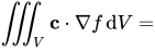
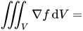
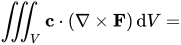
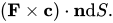
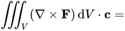
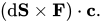
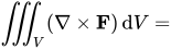
• スカラー関数gとベクトル場Fの場合、 ${\displaystyle \mathbf {F} \rightarrow \mathbf {F} g}$

${\displaystyle \iiint _{V}\left[\mathbf {F} \cdot \left(\nabla g\right)+g\left(\nabla \cdot \mathbf {F} \right)\right]\mathrm {d} V=}$ ${\displaystyle \scriptstyle S}$ ${\displaystyle g\mathbf {F} \cdot \mathbf {n} \mathrm {d} S.}$

この特殊なケースは であり、この場合、定理はグリーン恒等式の基礎となります。 ${\displaystyle \mathbf {F} =\nabla f}$

• 2つのベクトル場FとGに対して、外積を表す。 ${\displaystyle \mathbf {F} \rightarrow \mathbf {F} \times \mathbf {G} }$ ${\displaystyle \times }$

${\displaystyle \iiint _{V}\nabla \cdot \left(\mathbf {F} \times \mathbf {G} \right)\mathrm {d} V=\iiint _{V}\left[\mathbf {G} \cdot \left(\nabla \times \mathbf {F} \right)-\mathbf {F} \cdot \left(\nabla \times \mathbf {G} \right)\right]\,\mathrm {d} V=}$ ${\displaystyle \scriptstyle S}$ ${\displaystyle (\mathbf {F} \times \mathbf {G} )\cdot \mathbf {n} \mathrm {d} S.}$

• 2つのベクトル場FとGに対して、 はドット積を表す。 ${\displaystyle \mathbf {F} \rightarrow \mathbf {F} \cdot \mathbf {G} }$ ${\displaystyle \cdot }$

${\displaystyle \iiint _{V}\nabla \left(\mathbf {F} \cdot \mathbf {G} \right)\mathrm {d} V=\iiint _{V}\left[\left(\nabla \mathbf {G} \right)\cdot \mathbf {F} +\left(\nabla \mathbf {F} \right)\cdot \mathbf {G} \right]\,\mathrm {d} V=}$ ${\displaystyle \scriptstyle S}$ ${\displaystyle (\mathbf {F} \cdot \mathbf {G} )\mathbf {n} \mathrm {d} S.}$

• スカラー関数fとベクトル場cの場合：^[11] ${\displaystyle \mathbf {F} \rightarrow f\mathbf {c} }$  

${\displaystyle \iiint _{V}\mathbf {c} \cdot \nabla f\,\mathrm {d} V=}$ ${\displaystyle \scriptstyle S}$ ${\displaystyle (\mathbf {c} f)\cdot \mathbf {n} \mathrm {d} S-\iiint _{V}f(\nabla \cdot \mathbf {c} )\,\mathrm {d} V.}$

右側の最後の項は、定数または任意の発散のない（ソレノイド）ベクトル場、例えば相変化や化学反応などのソースやシンクのない非圧縮性の流れに対してはゼロになります。特に、定数とすると： ${\displaystyle \mathbf {c} }$ ${\displaystyle \mathbf {c} }$

${\displaystyle \iiint _{V}\nabla f\,\mathrm {d} V=}$ ${\displaystyle \scriptstyle S}$ ${\displaystyle f\mathbf {n} \mathrm {d} S.}$

• ベクトル場Fと定数ベクトルcの場合：^[11] ${\displaystyle \mathbf {F} \rightarrow \mathbf {c} \times \mathbf {F} }$

${\displaystyle \iiint _{V}\mathbf {c} \cdot (\nabla \times \mathbf {F} )\,\mathrm {d} V=}$ ${\displaystyle \scriptstyle S}$ ${\displaystyle (\mathbf {F} \times \mathbf {c} )\cdot \mathbf {n} \mathrm {d} S.}$

右辺の三重積を並べ替え、積分の定数ベクトルを取り出すと、

${\displaystyle \iiint _{V}(\nabla \times \mathbf {F} )\,\mathrm {d} V\cdot \mathbf {c} =}$ ${\displaystyle \scriptstyle S}$ ${\displaystyle (\mathrm {d} \mathbf {S} \times \mathbf {F} )\cdot \mathbf {c} .}$

したがって、

${\displaystyle \iiint _{V}(\nabla \times \mathbf {F} )\,\mathrm {d} V=}$ ${\displaystyle \scriptstyle S}$ ${\displaystyle \mathbf {n} \times \mathbf {F} \mathrm {d} S.}$

例

示された例に対応するベクトル場。ベクトルは球面内または球面外を指す場合があります。

発散定理は、左側の面のように、体積を完全に囲む閉面を通るフラックスを計算するために使用できます。ただし、右側の面のように境界を持つ面を通るフラックスを直接計算することはできません。（面は青、境界は赤で示されています。）

評価したいとします

${\displaystyle \scriptstyle S}$ ${\displaystyle \mathbf {F} \cdot \mathbf {n} \,\mathrm {d} S,}$

ここでSは次のように定義される単位球面である。

${\displaystyle S=\left\{(x,y,z)\in \mathbb {R} ^{3}\ :\ x^{2}+y^{2}+z^{2}=1\right\},}$

Fはベクトル場である

${\displaystyle \mathbf {F} =2x\mathbf {i} +y^{2}\mathbf {j} +z^{2}\mathbf {k} .}$

この積分の直接計算は非常に困難ですが、発散定理を使用すると結果の導出を簡略化できます。発散定理によれば、積分は次の式に等しいからです。

${\displaystyle \iiint _{W}(\nabla \cdot \mathbf {F} )\,\mathrm {d} V=2\iiint _{W}(1+y+z)\,\mathrm {d} V=2\iiint _{W}\mathrm {d} V+2\iiint _{W}y\,\mathrm {d} V+2\iiint _{W}z\,\mathrm {d} V,}$

ここでWは単位球である。

${\displaystyle W=\left\{(x,y,z)\in \mathbb {R} ^{3}\ :\ x^{2}+y^{2}+z^{2}\leq 1\right\}.}$

関数yはWの一方の半球面では正で、もう一方の半球面では負であり、等しく反対方向であるため、Wにおける全積分はゼロとなる。zについても同様である。

${\displaystyle \iiint _{W}y\,\mathrm {d} V=\iiint _{W}z\,\mathrm {d} V=0.}$

したがって、

${\displaystyle \scriptstyle S}$ ${\displaystyle \mathbf {F} \cdot \mathbf {n} \,\mathrm {d} S=2\iiint _{W}\,dV={\frac {8\pi }{3}},}$

単位球Wの体積 は⁠4π​/3⁠。

アプリケーション

物理法則の微分形式と積分形式

発散定理の結果として、多くの物理法則は微分形式（ある量が別の量の発散となる）と積分形式（ある量の閉曲面を通る流束が別の量に等しい）の両方で記述できます。例としては、ガウスの法則（静電気学）、磁気に関するガウスの法則、重力に関するガウスの法則が挙げられます。

連続方程式

連続方程式は、発散定理によって互いに関連付けられた、微分形式と積分形式の両方を持つ法則のより多くの例を提供します。流体力学、電磁気学、量子力学、相対性理論、その他多くの分野において、質量、運動量、エネルギー、確率、その他の量の保存を記述する連続方程式が存在します。一般的に、これらの方程式は、保存量の流れの発散が、その量のソースまたはシンクの分布に等しいことを述べています。発散定理は、そのような連続方程式はどれも、微分形式（発散の観点から）と積分形式（フラックスの観点から）で表すことができると述べています。^[12]

逆二乗則

逆二乗則は、ガウスの法則型の形式（前述のように微分積分形式を含む）で記述することができる。例としては、逆二乗クーロンの法則から導かれる静電気学におけるガウスの法則と、逆二乗ニュートンの万有引力の法則から導かれるガウスの重力の法則 が挙げられる。逆二乗定式からガウスの法則型方程式を導出する方法、あるいはその逆の方法は、どちらの場合も全く同じである。詳細は、それぞれの記事を参照のこと。^[12]

歴史

ジョゼフ＝ルイ・ラグランジュは1760年に面積分の概念を導入し、1811年には『解析力学』第2版でより一般的な用語で再び導入した。ラグランジュは流体力学の研究において面積分を用いた。^[13]彼は1762年に発散定理を発見した。^[14]

カール・フリードリヒ・ガウスも1813年に楕円体の引力に関する研究で面積分を使用し、発散定理の特殊な場合を証明しました。^{[15] [13]}彼は1833年と1839年にも追加の特殊な場合を証明しました^{。 [16]}しかし、1826年に熱の流れの研究の一環として一般定理の最初の証明を与えたのはミハイル・オストログラツキーでした。 ^[17]特殊な場合は、 1828年にジョージ・グリーンが「電気と磁気の理論への数学的分析の応用に関する論文」で証明しました。^{[18] [16]} シメオン・ドニ・ポアソンは1824年に弾性に関する論文で、フレデリック・サリュスは1828年に浮体に関する研究で証明しました。^{[19] [16]}

実例

例1

領域に対する発散定理の平面変形を検証するには： ${\displaystyle R}$

${\displaystyle R=\left\{(x,y)\in \mathbb {R} ^{2}\ :\ x^{2}+y^{2}\leq 1\right\},}$

そしてベクトル場：

${\displaystyle \mathbf {F} (x,y)=2y\mathbf {i} +5x\mathbf {j} .}$

の境界は単位円 であり、これは次のようにパラメータで表すことができます。 ${\displaystyle R}$ ${\displaystyle C}$

${\displaystyle x=\cos(s),\quad y=\sin(s)}$

となる。ただし単位は点から点までの弧の長さである。すると、のベクトル方程式は ${\displaystyle 0\leq s\leq 2\pi }$ ${\displaystyle s}$ ${\displaystyle s=0}$ ${\displaystyle P}$ ${\displaystyle C}$ ${\displaystyle C}$

${\displaystyle C(s)=\cos(s)\mathbf {i} +\sin(s)\mathbf {j} .}$

上の点において: ${\displaystyle P}$ ${\displaystyle C}$

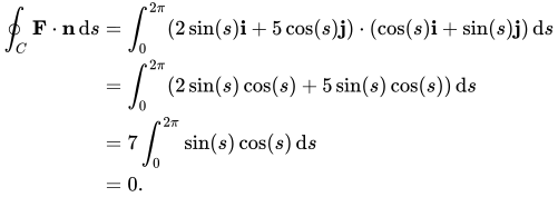
${\displaystyle P=(\cos(s),\,\sin(s))\,\Rightarrow \,\mathbf {F} =2\sin(s)\mathbf {i} +5\cos(s)\mathbf {j} .}$

したがって、

${\displaystyle {\begin{aligned}\oint _{C}\mathbf {F} \cdot \mathbf {n} \,\mathrm {d} s&=\int _{0}^{2\pi }(2\sin(s)\mathbf {i} +5\cos(s)\mathbf {j} )\cdot (\cos(s)\mathbf {i} +\sin(s)\mathbf {j} )\,\mathrm {d} s\\&=\int _{0}^{2\pi }(2\sin(s)\cos(s)+5\sin(s)\cos(s))\,\mathrm {d} s\\&=7\int _{0}^{2\pi }\sin(s)\cos(s)\,\mathrm {d} s\\&=0.\end{aligned}}}$

なので、 を評価することができ、なので、 を評価することができます。したがって、 ${\displaystyle M={\mathfrak {Re}}(\mathbf {F} )=2y}$ ${\displaystyle {\frac {\partial M}{\partial x}}=0}$ ${\displaystyle N={\mathfrak {Im}}(\mathbf {F} )=5x}$ ${\displaystyle {\frac {\partial N}{\partial y}}=0}$

${\displaystyle \iint _{R}\,\mathbf {\nabla } \cdot \mathbf {F} \,\mathrm {d} A=\iint _{R}\left({\frac {\partial M}{\partial x}}+{\frac {\partial N}{\partial y}}\right)\,\mathrm {d} A=0.}$

例2

次の不等式によって制限される次のベクトル場のフラックスを評価したいとします。 ${\displaystyle \mathbf {F} =2x^{2}{\textbf {i}}+2y^{2}{\textbf {j}}+2z^{2}{\textbf {k}}}$

${\displaystyle \left\{0\leq x\leq 3\right\},\left\{-2\leq y\leq 2\right\},\left\{0\leq z\leq 2\pi \right\}}$

発散定理によれば、

${\displaystyle \iiint _{V}\left(\mathbf {\nabla } \cdot \mathbf {F} \right)\mathrm {d} V=}$ ${\displaystyle \scriptstyle S}$ ${\displaystyle (\mathbf {F} \cdot \mathbf {n} )\,\mathrm {d} S.}$

ここで、 の発散を決定する必要があります。 が3次元ベクトル場である場合、 の発散はで与えられます。 ${\displaystyle {\textbf {F}}}$ ${\displaystyle \mathbf {F} }$ ${\displaystyle {\textbf {F}}}$ ${\textstyle \nabla \cdot {\textbf {F}}=\left({\frac {\partial }{\partial x}}{\textbf {i}}+{\frac {\partial }{\partial y}}{\textbf {j}}+{\frac {\partial }{\partial z}}{\textbf {k}}\right)\cdot {\textbf {F}}}$

したがって、次のフラックス積分を次のように設定できます。 ${\displaystyle I=}$ ${\displaystyle {\scriptstyle S}}$ ${\displaystyle \mathbf {F} \cdot \mathbf {n} \,\mathrm {d} S,}$

${\displaystyle {\begin{aligned}I&=\iiint _{V}\nabla \cdot \mathbf {F} \,\mathrm {d} V\\[6pt]&=\iiint _{V}\left({\frac {\partial \mathbf {F_{x}} }{\partial x}}+{\frac {\partial \mathbf {F_{y}} }{\partial y}}+{\frac {\partial \mathbf {F_{z}} }{\partial z}}\right)\mathrm {d} V\\[6pt]&=\iiint _{V}(4x+4y+4z)\,\mathrm {d} V\\[6pt]&=\int _{0}^{3}\int _{-2}^{2}\int _{0}^{2\pi }(4x+4y+4z)\,\mathrm {d} V\end{aligned}}}$

積分を設定したので、それを評価できます。

${\displaystyle {\begin{aligned}\int _{0}^{3}\int _{-2}^{2}\int _{0}^{2\pi }(4x+4y+4z)\,\mathrm {d} V&=\int _{-2}^{2}\int _{0}^{2\pi }(12y+12z+18)\,\mathrm {d} y\,\mathrm {d} z\\[6pt]&=\int _{0}^{2\pi }24(2z+3)\,\mathrm {d} z\\[6pt]&=48\pi (2\pi +3)\end{aligned}}}$

一般化

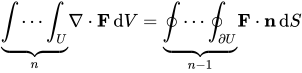
多次元

一般化されたストークスの定理を用いると、領域U上のベクトル場Fの発散のn次元体積積分を、Uの境界上のFの( n − 1)次元面積分と等しくすることができる。

${\displaystyle \underbrace {\int \cdots \int _{U}} _{n}\nabla \cdot \mathbf {F} \,\mathrm {d} V=\underbrace {\oint _{}\cdots \oint _{\partial U}} _{n-1}\mathbf {F} \cdot \mathbf {n} \,\mathrm {d} S}$

この方程式は発散定理としても知られています。

n = 2の場合、これはグリーンの定理と同等になります。

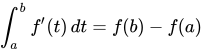
n = 1 のとき、これは微積分学の基本定理、第 2 部に帰着します。

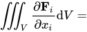
テンソル場

定理をアインシュタイン記法で書くと：

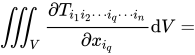
${\displaystyle \iiint _{V}{\dfrac {\partial \mathbf {F} _{i}}{\partial x_{i}}}\mathrm {d} V=}$ ${\displaystyle \scriptstyle S}$ ${\displaystyle \mathbf {F} _{i}n_{i}\,\mathrm {d} S}$

示唆的に、ベクトル場Fをn階テンソル場Tに置き換えると、これは次のように一般化できる。^[20]

${\displaystyle \iiint _{V}{\dfrac {\partial T_{i_{1}i_{2}\cdots i_{q}\cdots i_{n}}}{\partial x_{i_{q}}}}\mathrm {d} V=}$ ${\displaystyle \scriptstyle S}$ ${\displaystyle T_{i_{1}i_{2}\cdots i_{q}\cdots i_{n}}n_{i_{q}}\,\mathrm {d} S.}$

ここで、各辺において少なくとも1つの添え字に対してテンソル収縮が起こります。この定理の形は3次元においても成立し、各添え字は1、2、3の値を取ります。この定理はさらに高次元（または低次元）（例えば一般相対論における4次元時空^[21]）に一般化できます。

参照

• ケルビン・ストークスの定理
• 一般化ストークス定理
• 微分形式

参考文献

1. Katz, Victor J. (1979). 「ストークスの定理の歴史」.数学雑誌. 52 (3): 146– 156. doi :10.2307/2690275. JSTOR  2690275.アンダーソン、マーロウ（2009年）『イプシロンを授けたのは誰か？：その他の数学史物語』アメリカ数学会、  78～ 79頁に再録。ISBN 978-0-88385-569-0。
2. RGラーナー、GLトリッグ（1994年）。『物理学百科事典』（第2版）。VHC。ISBN 978-3-527-26954-9。
3. バイロン、フレデリック、フラー、ロバート（1992）、古典物理学と量子物理学の数学、ドーバー出版、p. 22、ISBN 978-0-486-67164-2
4. Wiley, C. Ray Jr.上級工学数学、第3版、McGraw-Hill、pp.  372– 373。
5. クレイシグ, エルウィン; クレイシグ, ハーバート; ノーミントン, エドワード J. (2011). 先端工学数学 (第10版). ジョン・ワイリー・アンド・サンズ. pp.  453– 456. ISBN 978-0-470-45836-5。
6. Benford, Frank A. (2007年5月). 「ベクトル微積分に関するノート」(PDF) .数学105：多変数微積分 のコース教材. ウィリアムズ大学 スティーブン・ミラー教授のウェブページ. 2022年3月14日閲覧.
7. パーセル、エドワード・M.、デイヴィッド・J・モーリン（2013年）『電気と磁気』ケンブリッジ大学出版局、pp.  56– 58. ISBN 978-1-107-01402-2。
8. Alt, Hans Wilhelm (2016). 「線形関数解析」. Universitext . ロンドン: Springer London. pp.  259– 261, 270– 272. doi :10.1007/978-1-4471-7280-2. ISBN 978-1-4471-7279-6. ISSN  0172-5939.
9. テイラー、マイケル・E. (2011). 「偏微分方程式 I」.応用数学科学. 第115巻. ニューヨーク: シュプリンガー・ニューヨーク. pp.  178– 179. doi :10.1007/978-1-4419-7055-8. ISBN 978-1-4419-7054-1. ISSN  0066-5452.
10. MRシュピーゲル; S. リプシュッツ; D. スペルマン (2009)。ベクトル解析。シャウムの概要（第 2 版）。アメリカ：マグロウヒル。ISBN 978-0-07-161545-7。
11. MathWorld
12. CB Parker (1994). McGraw Hill Encyclopaedia of Physics (第2版). McGraw Hill. ISBN 978-0-07-051400-3。
13. Katz, Victor (2009). 「第22章 ベクトル解析」. 『数学史入門』 . Addison-Wesley. pp.  808–9 . ISBN 978-0-321-38700-4。
14. ラグランジュは音に関する 1762 年の論文で、発散定理の特殊なケースを扱っています: Lagrange (1762) "Nouvelles recherches sur la Nature et la propagation duson" (音の性質と伝播に関する新しい研究)、Miscellanea Taurinensia (別名: Mélanges de Turin )、2 : 11 – 172。この記事は次のように再版されます。 「自然と伝播の新研究」、JA Serret 編、Oeuvres de Lagrange、(パリ、フランス: Gauthier-Villars、1867)、vol. 1、151～316ページ。 263 ～ 265 ページで、ラグランジュは部分積分を使用して三重積分を二重積分に変換します。
15. CF Gauss (1813) 「Theoria Attractis corporum sphaeroicorum ellipticorum homogeneorum methodo nova tractata」、Commentationes societatis regiae scientiarium Gottingensiscentiores、2 : 355–378;ガウスは定理の特殊な場合を考えました。彼の記事の 4、5、6 ページを参照してください。
16. Katz, Victor (1979年5月). 「ストークスの定理の歴史」.数学雑誌. 52 (3): 146– 156. doi :10.1080/0025570X.1979.11976770. JSTOR  2690275.
17. ミハイル・オストラグラツキーは1826年にパリ・アカデミーに発散定理の証明を提出したが、その研究はアカデミーによって出版されなかった。彼はロシアのサンクトペテルブルクに戻り、1828年から1829年にかけてフランスで行った研究をサンクトペテルブルク・アカデミーで発表した。アカ​​デミーは1831年に彼の研究を短縮形で出版した。
    • 彼が1826年2月13日にパリ・アカデミーで発表した発散定理の証明「積分学における定理の証明」（Démondstration d'un théorème du calcul intégral）は、1965年に彼自身の別の論文と共にロシア語に翻訳されました。参照：Юшкевич А.П. (Yushkevich AP) およびАнтропова В.И. (アントロポフ VI) (1965) 「Неопубликованные работы М.В. Остроградского」（MV Ostrogradskii の未発表作品）、Историко-математические исследования (Istoriko-Matematicheskie Isledovaniya / 歴史数学研究)、16 : 49–96; 「Остроградский М.В. Доказательство одной теоремы интегрального исчисления」というタイトルのセクションを参照してください。 Ostragradsky MV 積分微積分における定理の証明)。
    • M. Ostrogradsky (発表: 1828 年 11 月 5 日; 出版: 1831 年) 「Première note sur la théorie de la Chaleur」 (熱理論に関する最初のメモ) Mémoires de l'Académie impériale des Sciences de St. Pétersbourg、シリーズ 6、1 : 129–133。発散定理の彼の証明の短縮版については、130 ～ 131 ページを参照してください。
    • Victor J. Katz (1979年5月)「ストークスの定理の歴史」、2015年4月2日アーカイブ、Wayback Machineにて公開 。Mathematics Magazine、52 (3): 146–156 doi :10.1080/0025570X.1979.11976770。オストラグラツキーによる発散定理の証明については、147～148ページを参照。
18. ジョージ・グリーン著『電気と磁気の理論への数学的解析の応用に関するエッセイ』（ノッティンガム、イギリス：T. Wheelhouse、1838年）。「発散定理」の一形式は10～12ページに掲載されている。
19. 発散定理の何らかの形を使用した他の初期の研究者には次のような人々がいる。
    • ポアソン（発表：1824年2月2日、出版：1826年）「磁気理論に関する覚書」（Mémoire sur la théorie du magnétisme）、『Mémoires de l'Académie des sciences de l'Institut de France』、5 : 247–338。294–296ページで、ポアソンは体積積分（量Qの評価に用いられる）を面積積分に変換している。この変換を行うために、ポアソンは発散定理を証明するのと同じ手順に従った。
    • Frédéric Sarrus (1828) 「Mémoire sur les oscillations des corps flottans」（浮遊体の振動に関する回想録）、Annales de mathématiques pures et appliquées (Nismes)、19 : 185–211。
20. KF Riley、MP Hobson、SJ Bence (2010).物理学と工学のための数学的手法. ケンブリッジ大学出版局. ISBN 978-0-521-86153-3。
21. 例えば、 JA Wheeler、C. Misner、KS Thorne (1973). Gravitation . WH Freeman & Co. pp.  85– 86, §3.5. ISBNを参照
     978-0-7167-0344-0。、R.ペンローズ（2007年）『現実への道』ヴィンテージブックス。ISBN
     978-0-679-77631-4。

外部リンク

• 「オストログラツキの公式」数学百科事典、EMSプレス、2001 [1994]
• MathPagesの微分作用素と発散定理
• Nick Bykov による発散 (ガウス) 定理、Wolfram Demonstrations Project。
• ワイスタイン、エリック・W.「ダイバージェンス定理」。マスワールド。– この記事は元々、PlanetMathのGFDL記事(https://web.archive.org/web/20021029094728/http://planetmath.org/encyclopedia/Divergence.html)に基づいています。

Retrieved from "https://en.wikipedia.org/w/index.php?title=Divergence_theorem&oldid=1322212376"