Method of integration for rational functions
オイラー置換は 、次のような積分を評価する方法である。
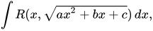
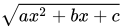
∫ R ( x , a x 2 + b x + c ) d x , {\displaystyle \int R(x,{\sqrt {ax^{2}+bx+c}})\,dx,}
ここで、は および の 有理関数 である 。これらの積分は常に3つのオイラー置換のいずれかを用いて有理化できることが証明されている。 [1] R {\displaystyle R} x {\displaystyle x} a x 2 + b x + c {\textstyle {\sqrt {ax^{2}+bx+c}}}
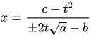
オイラーの第一置換 オイラーの第一置換は、 のときに用いられます 。 を代入して 、得られた式を解きます 。 となり、 項は において有理的に表現可能である ことがわかります a > 0 {\displaystyle a>0} a x 2 + b x + c = ± x a + t {\displaystyle {\sqrt {ax^{2}+bx+c}}=\pm x{\sqrt {a}}+t} x {\displaystyle x} x = c − t 2 ± 2 t a − b {\displaystyle x={\frac {c-t^{2}}{\pm 2t{\sqrt {a}}-b}}} d x {\displaystyle dx} t {\displaystyle t}
この置換では、正の符号または負の符号のいずれかを選択できます。
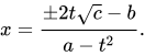
オイラーの第二置換 の場合 、 を取ります。 上と同様 に を解くと、 c > 0 {\displaystyle c>0} a x 2 + b x + c = x t ± c . {\displaystyle {\sqrt {ax^{2}+bx+c}}=xt\pm {\sqrt {c}}.} x {\displaystyle x} x = ± 2 t c − b a − t 2 . {\displaystyle x={\frac {\pm 2t{\sqrt {c}}-b}{a-t^{2}}}.}
ここでも、正負の符号のいずれかを選択できます。
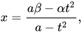
オイラーの第三置換 多項式が 実根を持ち 、の場合 、 を選択できます 。これにより となり 、前の場合と同様に、被積分関数全体を で有理的に表すことができ ます a x 2 + b x + c {\displaystyle ax^{2}+bx+c} α {\displaystyle \alpha } β {\displaystyle \beta } a x 2 + b x + c = a ( x − α ) ( x − β ) = ( x − α ) t {\textstyle {\sqrt {ax^{2}+bx+c}}={\sqrt {a(x-\alpha )(x-\beta )}}=(x-\alpha )t} x = a β − α t 2 a − t 2 , {\displaystyle x={\frac {a\beta -\alpha t^{2}}{a-t^{2}}},} t {\displaystyle t}
例
オイラーの第一置換の例
最初の例 積分 については 、最初の置換法を用いて と設定することができる 。したがって、 以下の式が得られる。 ∫ d x x 2 + c {\displaystyle \int \!{\frac {\ dx}{\sqrt {x^{2}+c}}}} x 2 + c = − x + t {\textstyle {\sqrt {x^{2}+c}}=-x+t} x = t 2 − c 2 t , d x = t 2 + c 2 t 2 d t , {\displaystyle x={\frac {t^{2}-c}{2t}},\qquad \ dx={\frac {t^{2}+c}{2t^{2}}}\,\ dt,} x 2 + c = − t 2 − c 2 t + t = t 2 + c 2 t . {\displaystyle {\sqrt {x^{2}+c}}=-{\frac {t^{2}-c}{2t}}+t={\frac {t^{2}+c}{2t}}.} ∫ d x x 2 + c = ∫ t 2 + c 2 t 2 t 2 + c 2 t d t = ∫ d t t = ln | t | + C = ln | x + x 2 + c | + C . {\displaystyle \int {\frac {dx}{\sqrt {x^{2}+c}}}=\int {\frac {\frac {t^{2}+c}{2t^{2}}}{\frac {t^{2}+c}{2t}}}\,\ dt=\int {\frac {dt}{t}}=\ln |t|+C=\ln \left|x+{\sqrt {x^{2}+c}}\right|+C.}
事例から 式がわかる c = ± 1 {\displaystyle c=\pm 1} ∫ d x x 2 + 1 = arsinh ( x ) + C , ∫ d x x 2 − 1 = arcosh ( x ) + C . ( x > 1 ) {\displaystyle {\begin{aligned}\int {\frac {\ dx}{\sqrt {x^{2}+1}}}&=\operatorname {arsinh} (x)+C,\\[6pt]\int {\frac {\ dx}{\sqrt {x^{2}-1}}}&=\operatorname {arcosh} (x)+C.\qquad (x>1)\end{aligned}}}
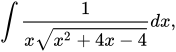
2番目の例 の値を求めるには、 オイラーの最初の代入法を使って
次のように求めます 。両辺を2乗すると となり 、そこから 項が打ち消されます。 を解く と ∫ 1 x x 2 + 4 x − 4 d x , {\displaystyle \int {\frac {1}{x{\sqrt {x^{2}+4x-4}}}}dx,} t {\displaystyle t} x 2 + 4 x − 4 = 1 x + t = x + t {\textstyle {\sqrt {x^{2}+4x-4}}={\sqrt {1}}x+t=x+t} x 2 + 4 x − 4 = x 2 + 2 x t + t 2 {\displaystyle x^{2}+4x-4=x^{2}+2xt+t^{2}} x 2 {\displaystyle x^{2}} x {\displaystyle x} x = t 2 + 4 4 − 2 t . {\displaystyle x={\frac {t^{2}+4}{4-2t}}.}
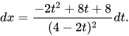
そこから、微分 とは 次の関係にある
ことがわかります。 d x {\displaystyle dx} d t {\displaystyle dt} d x = − 2 t 2 + 8 t + 8 ( 4 − 2 t ) 2 d t . {\displaystyle dx={\frac {-2t^{2}+8t+8}{(4-2t)^{2}}}dt.}
したがって、 ∫ d x x x 2 + 4 x − 4 = ∫ − 2 t 2 + 8 t + 8 ( 4 − 2 t ) 2 ( t 2 + 4 4 − 2 t ) ( − t 2 + 4 t + 4 4 − 2 t ) d t t = x 2 + 4 x − 4 − x = 2 ∫ d t t 2 + 4 = tan − 1 ( t 2 ) + C = tan − 1 ( x 2 + 4 x − 4 − x 2 ) + C . {\displaystyle {\begin{aligned}\int {\frac {dx}{x{\sqrt {x^{2}+4x-4}}}}&=\int {\frac {\frac {-2t^{2}+8t+8}{(4-2t)^{2}}}{\left({\frac {t^{2}+4}{4-2t}}\right)\left({\frac {-t^{2}+4t+4}{4-2t}}\right)}}dt&&t={\sqrt {x^{2}+4x-4}}-x\\[6pt]&=2\int {\frac {dt}{t^{2}+4}}=\tan ^{-1}\left({\frac {t}{2}}\right)+C\\[6pt]&=\tan ^{-1}\left({\frac {{\sqrt {x^{2}+4x-4}}-x}{2}}\right)+C.\end{aligned}}}
オイラーの2番目の置換の例 積分では
、2番目の置換を使用して設定できます 。したがって 、 ∫ d x x − x 2 + x + 2 , {\displaystyle \int \!{\frac {dx}{x{\sqrt {-x^{2}+x+2}}}},} − x 2 + x + 2 = x t + 2 {\displaystyle {\sqrt {-x^{2}+x+2}}=xt+{\sqrt {2}}} x = 1 − 2 2 t t 2 + 1 , d x = 2 2 t 2 − 2 t − 2 2 ( t 2 + 1 ) 2 d t , {\displaystyle x={\frac {1-2{\sqrt {2}}t}{t^{2}+1}},\qquad dx={\frac {2{\sqrt {2}}t^{2}-2t-2{\sqrt {2}}}{(t^{2}+1)^{2}}}dt,} − x 2 + x + 2 = 1 − 2 2 t t 2 + 1 t + 2 = − 2 t 2 + t + 2 t 2 + 1 . {\displaystyle {\sqrt {-x^{2}+x+2}}={\frac {1-2{\sqrt {2}}t}{t^{2}+1}}t+{\sqrt {2}}={\frac {-{\sqrt {2}}t^{2}+t+{\sqrt {2}}}{t^{2}+1}}.}
したがって、次の式が得られます。 ∫ d x x − x 2 + x + 2 = ∫ 2 2 t 2 − 2 t − 2 2 ( t 2 + 1 ) 2 1 − 2 2 t t 2 + 1 − 2 t 2 + t + 2 t 2 + 1 d t = ∫ − 2 − 2 2 t + 1 d t = 1 2 ∫ − 2 2 − 2 2 t + 1 d t = 1 2 ln | 2 2 t − 1 | + C = 2 2 ln | 2 2 − x 2 + x + 2 − 2 x − 1 | + C . {\displaystyle {\begin{aligned}\int {\frac {dx}{x{\sqrt {-x^{2}+x+2}}}}&=\int {\frac {\frac {2{\sqrt {2}}t^{2}-2t-2{\sqrt {2}}}{(t^{2}+1)^{2}}}{{\frac {1-2{\sqrt {2}}t}{t^{2}+1}}{\frac {-{\sqrt {2}}t^{2}+t+{\sqrt {2}}}{t^{2}+1}}}}dt\\[6pt]&=\int \!{\frac {-2}{-2{\sqrt {2}}t+1}}dt={\frac {1}{\sqrt {2}}}\int {\frac {-2{\sqrt {2}}}{-2{\sqrt {2}}t+1}}dt\\[6pt]&={\frac {1}{\sqrt {2}}}\ln \left|2{\sqrt {2}}t-1\right|+C\\[4pt]&={\frac {\sqrt {2}}{2}}\ln \left|2{\sqrt {2}}{\frac {{\sqrt {-x^{2}+x+2}}-{\sqrt {2}}}{x}}-1\right|+C.\end{aligned}}}
オイラーの3番目の置換の例 評価するには
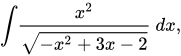
、3番目の置換を使用して設定します 。したがって 、 ∫ x 2 − x 2 + 3 x − 2 d x , {\displaystyle \int \!{\frac {x^{2}}{\sqrt {-x^{2}+3x-2}}}\ dx,} − ( x − 2 ) ( x − 1 ) = ( x − 2 ) t {\textstyle {\sqrt {-(x-2)(x-1)}}=(x-2)t} x = − 2 t 2 − 1 − t 2 − 1 , d x = 2 t ( − t 2 − 1 ) 2 d t , {\displaystyle x={\frac {-2t^{2}-1}{-t^{2}-1}},\qquad \ dx={\frac {2t}{(-t^{2}-1)^{2}}}\,\ dt,} − x 2 + 3 x − 2 = ( x − 2 ) t = t − t 2 − 1. . {\displaystyle {\sqrt {-x^{2}+3x-2}}=(x-2)t={\frac {t}{-t^{2}-1.}}.}
次に、 これは有理関数であり、部分分数を使用して解くことができます。 ∫ x 2 − x 2 + 3 x − 2 d x = ∫ ( − 2 t 2 − 1 − t 2 − 1 ) 2 2 t ( − t 2 − 1 ) 2 t − t 2 − 1 d t = ∫ 2 ( − 2 t 2 − 1 ) 2 ( − t 2 − 1 ) 3 d t . {\displaystyle \int {\frac {x^{2}}{\sqrt {-x^{2}+3x-2}}}\ dx=\int {\frac {\left({\frac {-2t^{2}-1}{-t^{2}-1}}\right)^{2}{\frac {2t}{(-t^{2}-1)^{2}}}}{\frac {t}{-t^{2}-1}}}\ dt=\int {\frac {2(-2t^{2}-1)^{2}}{(-t^{2}-1)^{3}}}\ dt.}
一般化 オイラーの置換法は、虚数の使用を許可することで一般化できます。例えば、積分では 置換法 を使用できます。複素数への拡張により、二次式の係数に関係なく、あらゆる種類のオイラー置換法を使用できます ∫ d x − x 2 + c {\textstyle \int {\frac {dx}{\sqrt {-x^{2}+c}}}} − x 2 + c = ± i x + t {\textstyle {\sqrt {-x^{2}+c}}=\pm ix+t}
オイラーの置換法は、より広い関数のクラスに一般化できます。 の形の積分を考えてみましょう
。 ここで 、 とは それぞれの 有理関数です。 この積分は、 の置換によって 別の積分に
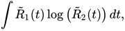
変換できます。この 場合 、 と は単に の有理関数となります 。原理的には、 因数分解 と 部分分数分解を用いて積分を単純な項に分解し、二 重対数 関数を用いて解析的に積分することができます 。 [2] ∫ R 1 ( x , a x 2 + b x + c ) log ( R 2 ( x , a x 2 + b x + c ) ) d x , {\displaystyle \int R_{1}\left(x,{\sqrt {ax^{2}+bx+c}}\right)\,\log \left(R_{2}\left(x,{\sqrt {ax^{2}+bx+c}}\right)\right)\,dx,} R 1 {\displaystyle R_{1}} R 2 {\displaystyle R_{2}} x {\displaystyle x} a x 2 + b x + c {\textstyle {\sqrt {ax^{2}+bx+c}}} a x 2 + b x + c = a + x t {\textstyle {\sqrt {ax^{2}+bx+c}}={\sqrt {a}}+xt} ∫ R ~ 1 ( t ) log ( R ~ 2 ( t ) ) d t , {\displaystyle \int {\tilde {R}}_{1}(t)\log {\big (}{\tilde {R}}_{2}(t){\big )}\,dt,} R ~ 1 ( t ) {\displaystyle {\tilde {R}}_{1}(t)} R ~ 2 ( t ) {\displaystyle {\tilde {R}}_{2}(t)} t {\displaystyle t}
参照
参考文献 ^ N. Piskunov, Diferentsiaal- ja integraalarvutus körgematele tehnilistele öppeasutustele. Viies, taiendatud trukk. Kirjastus Valgus , Tallinn (1965). 注:オイラー置換はほとんどのロシアの微積分学の教科書に掲載されています ^ ダニエル・ズウィリンガー著 『統合ハンドブック 』ジョーンズ・アンド・バートレット共著、 145~ 146頁 。ISBN 978-0867202939 。 この記事には、 PlanetMath の「Eulers Substitutions For Integration」の資料が組み込まれており 、 クリエイティブ・コモンズの表示/継承ライセンスの下でライセンスされています
















![{\displaystyle {\begin{aligned}\int {\frac {\dx}{\sqrt {x^{2}+1}}}&=\operatorname {arsinh} (x)+C,\\[6pt]\int {\frac {\dx}{\sqrt {x^{2}-1}}}&=\operatorname {arcosh} (x)+C.\qquad (x>1)\end{aligned}}}](https://wikimedia.org/api/rest_v1/media/math/render/svg/09dffcdf79626c1f669201cbd38b4a2236b47030)




![{\displaystyle {\begin{aligned}\int {\frac {dx}{x{\sqrt {x^{2}+4x-4}}}}&=\int {\frac {\frac {-2t^{2}+8t+8}{(4-2t)^{2}}}{\left({\frac {t^{2}+4}{4-2t}}\right)\left({\frac {-t^{2}+4t+4}{4-2t}}\right)}}dt&&t={\sqrt {x^{2}+4x-4}}-x\\[6pt]&=2\int {\frac {dt}{t^{2}+4}}=\tan ^{-1}\left({\frac {t}{2}}\right)+C\\[6pt]&=\tan ^{-1}\left({\frac {{\sqrt {x^{2}+4x-4}}-x}{2}}\right)+C.\end{aligned}}}](https://wikimedia.org/api/rest_v1/media/math/render/svg/020e1b2f7881b7b85ba1de808cc4b921b80cfc29)




![{\displaystyle {\begin{aligned}\int {\frac {dx}{x{\sqrt {-x^{2}+x+2}}}}&=\int {\frac {\frac {2{\sqrt {2}}t^{2}-2t-2{\sqrt {2}}}{(t^{2}+1)^{2}}}{{\frac {1-2{\sqrt {2}}t}{t^{2}+1}}{\frac {-{\sqrt {2}}t^{2}+t+{\sqrt {2}}}{t^{2}+1}}}}dt\\[6pt]&=\int \!{\frac {-2}{-2{\sqrt {2}}t+1}}dt={\frac {1}{\sqrt {2}}}\int {\frac {-2{\sqrt {2}}}{-2{\sqrt {2}}t+1}}dt\\[6pt]&={\frac {1}{\sqrt {2}}}\ln \left|2{\sqrt {2}}t-1\right|+C\\[4pt]&={\frac {\sqrt {2}}{2}}\ln \left|2{\sqrt {2}}{\frac {{\sqrt {-x^{2}+x+2}}-{\sqrt {2}}}{x}}-1\right|+C.\end{aligned}}}](https://wikimedia.org/api/rest_v1/media/math/render/svg/5a5148c46496eeafd07b4ee981f9b74282b924a7)